

11 Optical Diagnostics with Ultrafast and Strong Field Raman Techniques
277
thermal equilibrium, one has cos 2 θ p = 1/3 and cos 2 θ c = 0. After the coherent
excitation of the rotational levels, cos 2 θ p goes beyond the 1/3 isotropic value,
whereas cos 2 θ c = 0. In a non-dissipative media, cos 2 θ p remain constant, and
cos 2 θ c oscillates at the rotational period as long as the coherence is maintained,
but in presence of collisional relaxation, both decay to their equilibrium values.
If one makes the assumption of M-independent K J MJ M [38] (i.e., the orientation of the angular momentum is randomize by collisions), then the latter can be
constructed with the usual ECS approach [8] and Eq. (11.6) can be applied. Using
Eqs. (11.17)–(11.18), one can write
dcos 2 θ p (t)
dt
= −
J,M
γ J ρ J MJ M (t)V J MJ M +
J,M
J M
K J MJ M ρ J MJ M V J MJ M
(11.20)
and
dcos 2 θ c (t)
dt
= −
J =J ,M
1
2
[γ J + γ J ] + γ
(pd)
J J
ρ J MJ M V J MJ M
(11.21)
where V J MJ M are the elements of the cos 2 θ operator. In the case of CO 2 , the
collisional linewidths γ J only depend slightly on the J value, so that they can be
replaced by an averaged value γ .
As expected from Eqs. (11.20)–(11.21), cos 2 θ c should not decay at the same
rate as cos 2 θ p , the latter decreasing with a time constant of 1/γ , the former decaying with a time constant of 1/(γ + γ (pd) ) (if one replaces the γ
(pd)
J J by an averaged
value). Thus, it would be possible to experimentally evidence these two different
temporal decays, providing the contribution of γ
(pd)
J J term can be separately predicted.
Thanks to a classical approach [42, 43], it is indeed possible to disentangle the
elastic and inelastic contributions to the collisional linewidths, and then to construct
the relaxation rates by fitting the scaling laws mentioned in Sect. 11.2.1 on the inelastic part only. Comparing computed values of cos 2 θ (t) with experimental data
should therefore provides a way of questioning the calculated value of γ
(pd)
J J .
11.3.1.2 Experimental Procedure and Results
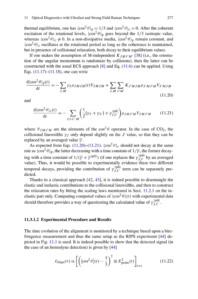
The time evolution of the alignment is monitored by a technique based upon a birefringence measurement and thus the same setup as the RIPS experiment [44] depicted in Fig. 11.1 is used. It is indeed possible to show that the detected signal (in
the case of an homodyne detection) is given by [44]
I Align (τ ) ∝
cos
2 θ
(t) −
1
3
2
⊗ E
2
probe (t)
t=τ
(11.22)
277
thermal equilibrium, one has cos 2 θ p = 1/3 and cos 2 θ c = 0. After the coherent
excitation of the rotational levels, cos 2 θ p goes beyond the 1/3 isotropic value,
whereas cos 2 θ c = 0. In a non-dissipative media, cos 2 θ p remain constant, and
cos 2 θ c oscillates at the rotational period as long as the coherence is maintained,
but in presence of collisional relaxation, both decay to their equilibrium values.
If one makes the assumption of M-independent K J MJ M [38] (i.e., the orientation of the angular momentum is randomize by collisions), then the latter can be
constructed with the usual ECS approach [8] and Eq. (11.6) can be applied. Using
Eqs. (11.17)–(11.18), one can write
dcos 2 θ p (t)
dt
= −
J,M
γ J ρ J MJ M (t)V J MJ M +
J,M
J M
K J MJ M ρ J MJ M V J MJ M
(11.20)
and
dcos 2 θ c (t)
dt
= −
J =J ,M
1
2
[γ J + γ J ] + γ
(pd)
J J
ρ J MJ M V J MJ M
(11.21)
where V J MJ M are the elements of the cos 2 θ operator. In the case of CO 2 , the
collisional linewidths γ J only depend slightly on the J value, so that they can be
replaced by an averaged value γ .
As expected from Eqs. (11.20)–(11.21), cos 2 θ c should not decay at the same
rate as cos 2 θ p , the latter decreasing with a time constant of 1/γ , the former decaying with a time constant of 1/(γ + γ (pd) ) (if one replaces the γ
(pd)
J J by an averaged
value). Thus, it would be possible to experimentally evidence these two different
temporal decays, providing the contribution of γ
(pd)
J J term can be separately predicted.
Thanks to a classical approach [42, 43], it is indeed possible to disentangle the
elastic and inelastic contributions to the collisional linewidths, and then to construct
the relaxation rates by fitting the scaling laws mentioned in Sect. 11.2.1 on the inelastic part only. Comparing computed values of cos 2 θ (t) with experimental data
should therefore provides a way of questioning the calculated value of γ
(pd)
J J .
11.3.1.2 Experimental Procedure and Results
The time evolution of the alignment is monitored by a technique based upon a birefringence measurement and thus the same setup as the RIPS experiment [44] depicted in Fig. 11.1 is used. It is indeed possible to show that the detected signal (in
the case of an homodyne detection) is given by [44]
I Align (τ ) ∝
cos
2 θ
(t) −
1
3
2
⊗ E
2
probe (t)
t=τ
(11.22)