

274
F. Chaussard et al.
Table 11.1 Thermometry procedure in H 2 –N 2 mixtures, using the KS-1D model (T KS−1D ), or
the Lorentzian limit without the speed-dependence of the collisional parameters (T Lorentz(1) ), or
with the speed-dependence of the collisional parameters (T Lorentz(2) ). The reference temperature is
measured by a thermocouple. The values in parentheses are standard deviations
H 2 –N 2
5 % H 2 , 95 % N 2
50 % H 2 , 50 % N 2
T Th
593
899
T Lorentz(1)
741(1)
929(8)
T Lorentz(2)
557(5)
864(7)
T KS-1D
602(5)
885(7)
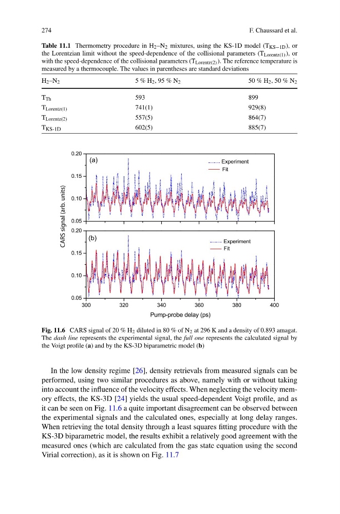
Fig. 11.6 CARS signal of 20 % H 2 diluted in 80 % of N 2 at 296 K and a density of 0.893 amagat.
The dash line represents the experimental signal, the full one represents the calculated signal by
the Voigt profile (a) and by the KS-3D biparametric model (b)
In the low density regime [26], density retrievals from measured signals can be
performed, using two similar procedures as above, namely with or without taking
into account the influence of the velocity effects. When neglecting the velocity memory effects, the KS-3D [24] yields the usual speed-dependent Voigt profile, and as
it can be seen on Fig. 11.6 a quite important disagreement can be observed between
the experimental signals and the calculated ones, especially at long delay ranges.
When retrieving the total density through a least squares fitting procedure with the
KS-3D biparametric model, the results exhibit a relatively good agreement with the
measured ones (which are calculated from the gas state equation using the second
Virial correction), as it is shown on Fig. 11.7
F. Chaussard et al.
Table 11.1 Thermometry procedure in H 2 –N 2 mixtures, using the KS-1D model (T KS−1D ), or
the Lorentzian limit without the speed-dependence of the collisional parameters (T Lorentz(1) ), or
with the speed-dependence of the collisional parameters (T Lorentz(2) ). The reference temperature is
measured by a thermocouple. The values in parentheses are standard deviations
H 2 –N 2
5 % H 2 , 95 % N 2
50 % H 2 , 50 % N 2
T Th
593
899
T Lorentz(1)
741(1)
929(8)
T Lorentz(2)
557(5)
864(7)
T KS-1D
602(5)
885(7)
Fig. 11.6 CARS signal of 20 % H 2 diluted in 80 % of N 2 at 296 K and a density of 0.893 amagat.
The dash line represents the experimental signal, the full one represents the calculated signal by
the Voigt profile (a) and by the KS-3D biparametric model (b)
In the low density regime [26], density retrievals from measured signals can be
performed, using two similar procedures as above, namely with or without taking
into account the influence of the velocity effects. When neglecting the velocity memory effects, the KS-3D [24] yields the usual speed-dependent Voigt profile, and as
it can be seen on Fig. 11.6 a quite important disagreement can be observed between
the experimental signals and the calculated ones, especially at long delay ranges.
When retrieving the total density through a least squares fitting procedure with the
KS-3D biparametric model, the results exhibit a relatively good agreement with the
measured ones (which are calculated from the gas state equation using the second
Virial correction), as it is shown on Fig. 11.7