

7 Ultrafast Laser-Induced Processes Described by Ab Initio Molecular
155
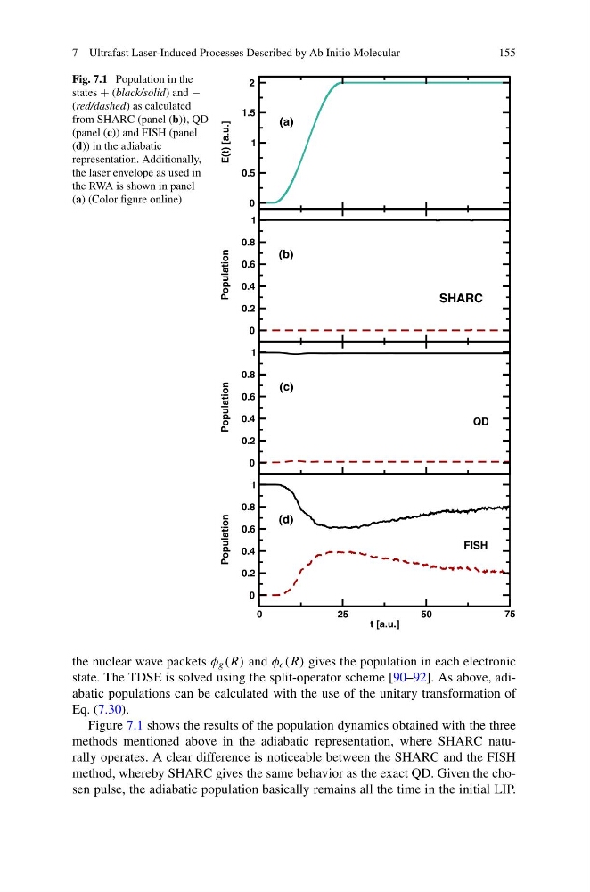
Fig. 7.1 Population in the
states + (black/solid) and −
(red/dashed) as calculated
from SHARC (panel (b)), QD
(panel (c)) and FISH (panel
(d)) in the adiabatic
representation. Additionally,
the laser envelope as used in
the RWA is shown in panel
(a) (Color figure online)
the nuclear wave packets φ g (R) and φ e (R) gives the population in each electronic
state. The TDSE is solved using the split-operator scheme [90–92]. As above, adiabatic populations can be calculated with the use of the unitary transformation of
Eq. (7.30).
Figure 7.1 shows the results of the population dynamics obtained with the three
methods mentioned above in the adiabatic representation, where SHARC naturally operates. A clear difference is noticeable between the SHARC and the FISH
method, whereby SHARC gives the same behavior as the exact QD. Given the chosen pulse, the adiabatic population basically remains all the time in the initial LIP.
155
Fig. 7.1 Population in the
states + (black/solid) and −
(red/dashed) as calculated
from SHARC (panel (b)), QD
(panel (c)) and FISH (panel
(d)) in the adiabatic
representation. Additionally,
the laser envelope as used in
the RWA is shown in panel
(a) (Color figure online)
the nuclear wave packets φ g (R) and φ e (R) gives the population in each electronic
state. The TDSE is solved using the split-operator scheme [90–92]. As above, adiabatic populations can be calculated with the use of the unitary transformation of
Eq. (7.30).
Figure 7.1 shows the results of the population dynamics obtained with the three
methods mentioned above in the adiabatic representation, where SHARC naturally operates. A clear difference is noticeable between the SHARC and the FISH
method, whereby SHARC gives the same behavior as the exact QD. Given the chosen pulse, the adiabatic population basically remains all the time in the initial LIP.