

154
L. González et al.
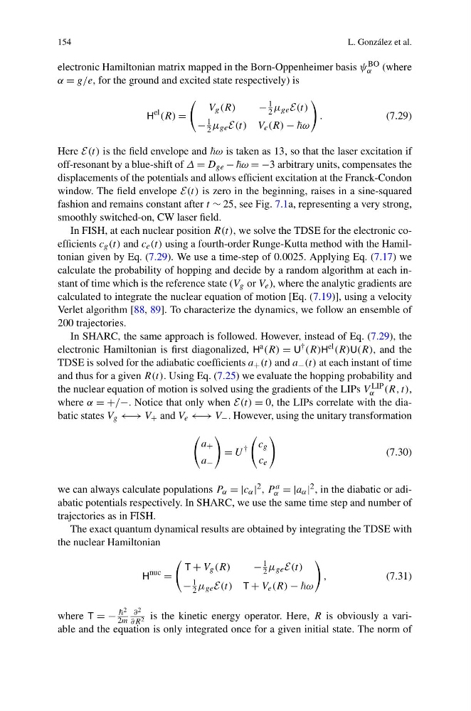
electronic Hamiltonian matrix mapped in the Born-Oppenheimer basis ψ BO
α (where
α = g/e, for the ground and excited state respectively) is
H
el (R) =
V g (R)
−
1
2 μ ge E(t)
−
1
2 μ ge E(t) V e (R) − ω
.
(7.29)
Here E(t) is the field envelope and ω is taken as 13, so that the laser excitation if
off-resonant by a blue-shift of Δ = D ge − ω = −3 arbitrary units, compensates the
displacements of the potentials and allows efficient excitation at the Franck-Condon
window. The field envelope E(t) is zero in the beginning, raises in a sine-squared
fashion and remains constant after t ∼ 25, see Fig. 7.1a, representing a very strong,
smoothly switched-on, CW laser field.
In FISH, at each nuclear position R(t), we solve the TDSE for the electronic coefficients c g (t) and c e (t) using a fourth-order Runge-Kutta method with the Hamiltonian given by Eq. (7.29). We use a time-step of 0.0025. Applying Eq. (7.17) we
calculate the probability of hopping and decide by a random algorithm at each instant of time which is the reference state (V g or V e ), where the analytic gradients are
calculated to integrate the nuclear equation of motion [Eq. (7.19)], using a velocity
Verlet algorithm [88, 89]. To characterize the dynamics, we follow an ensemble of
200 trajectories.
In SHARC, the same approach is followed. However, instead of Eq. (7.29), the
electronic Hamiltonian is first diagonalized, H a (R) = U † (R)H el (R)U(R), and the
TDSE is solved for the adiabatic coefficients a + (t) and a − (t) at each instant of time
and thus for a given R(t). Using Eq. (7.25) we evaluate the hopping probability and
the nuclear equation of motion is solved using the gradients of the LIPs V LIP
α (R, t),
where α = +/−. Notice that only when E(t) = 0, the LIPs correlate with the diabatic states V g ←→ V + and V e ←→ V − . However, using the unitary transformation
a +
a −
= U
†
c g
c e
(7.30)
we can always calculate populations P α = |c α | 2 , P a
α = |a α | 2 , in the diabatic or adiabatic potentials respectively. In SHARC, we use the same time step and number of
trajectories as in FISH.
The exact quantum dynamical results are obtained by integrating the TDSE with
the nuclear Hamiltonian
H
nuc
=
T + V g (R)
−
1
2 μ ge E(t)
−
1
2 μ ge E(t) T + V e (R) − ω
,
(7.31)
where T = −
2
2m
∂ 2
∂R 2 is the kinetic energy operator. Here, R is obviously a variable and the equation is only integrated once for a given initial state. The norm of
L. González et al.
electronic Hamiltonian matrix mapped in the Born-Oppenheimer basis ψ BO
α (where
α = g/e, for the ground and excited state respectively) is
H
el (R) =
V g (R)
−
1
2 μ ge E(t)
−
1
2 μ ge E(t) V e (R) − ω
.
(7.29)
Here E(t) is the field envelope and ω is taken as 13, so that the laser excitation if
off-resonant by a blue-shift of Δ = D ge − ω = −3 arbitrary units, compensates the
displacements of the potentials and allows efficient excitation at the Franck-Condon
window. The field envelope E(t) is zero in the beginning, raises in a sine-squared
fashion and remains constant after t ∼ 25, see Fig. 7.1a, representing a very strong,
smoothly switched-on, CW laser field.
In FISH, at each nuclear position R(t), we solve the TDSE for the electronic coefficients c g (t) and c e (t) using a fourth-order Runge-Kutta method with the Hamiltonian given by Eq. (7.29). We use a time-step of 0.0025. Applying Eq. (7.17) we
calculate the probability of hopping and decide by a random algorithm at each instant of time which is the reference state (V g or V e ), where the analytic gradients are
calculated to integrate the nuclear equation of motion [Eq. (7.19)], using a velocity
Verlet algorithm [88, 89]. To characterize the dynamics, we follow an ensemble of
200 trajectories.
In SHARC, the same approach is followed. However, instead of Eq. (7.29), the
electronic Hamiltonian is first diagonalized, H a (R) = U † (R)H el (R)U(R), and the
TDSE is solved for the adiabatic coefficients a + (t) and a − (t) at each instant of time
and thus for a given R(t). Using Eq. (7.25) we evaluate the hopping probability and
the nuclear equation of motion is solved using the gradients of the LIPs V LIP
α (R, t),
where α = +/−. Notice that only when E(t) = 0, the LIPs correlate with the diabatic states V g ←→ V + and V e ←→ V − . However, using the unitary transformation
a +
a −
= U
†
c g
c e
(7.30)
we can always calculate populations P α = |c α | 2 , P a
α = |a α | 2 , in the diabatic or adiabatic potentials respectively. In SHARC, we use the same time step and number of
trajectories as in FISH.
The exact quantum dynamical results are obtained by integrating the TDSE with
the nuclear Hamiltonian
H
nuc
=
T + V g (R)
−
1
2 μ ge E(t)
−
1
2 μ ge E(t) T + V e (R) − ω
,
(7.31)
where T = −
2
2m
∂ 2
∂R 2 is the kinetic energy operator. Here, R is obviously a variable and the equation is only integrated once for a given initial state. The norm of