

7 Ultrafast Laser-Induced Processes Described by Ab Initio Molecular
153
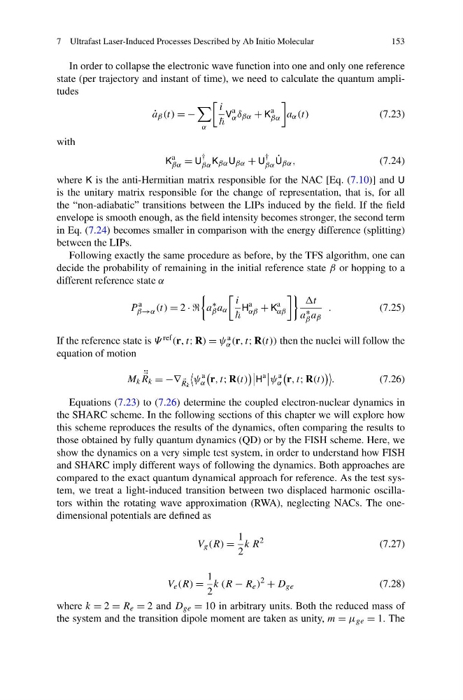
In order to collapse the electronic wave function into one and only one reference
state (per trajectory and instant of time), we need to calculate the quantum amplitudes
˙
a β (t) = −
α
i
V
a
α δ βα + K
a
βα
a α (t)
(7.23)
with
K
a
βα = U
†
βα K βα U βα + U
†
βα
˙
U βα ,
(7.24)
where K is the anti-Hermitian matrix responsible for the NAC [Eq. (7.10)] and U
is the unitary matrix responsible for the change of representation, that is, for all
the “non-adiabatic” transitions between the LIPs induced by the field. If the field
envelope is smooth enough, as the field intensity becomes stronger, the second term
in Eq. (7.24) becomes smaller in comparison with the energy difference (splitting)
between the LIPs.
Following exactly the same procedure as before, by the TFS algorithm, one can
decide the probability of remaining in the initial reference state β or hopping to a
different reference state α
P
a
β→α (t) = 2 · ·
a
∗
β a α
i
H
a
αβ + K
a
αβ
t
a ∗
β a β
.
(7.25)
If the reference state is Ψ ref (r, t; R) = ψ a
α (r, t; R(t)) then the nuclei will follow the
equation of motion
M k
¨
R k = −∇
R k
ψ
a
α
r, t; R(t)
H
a
ψ
a
α
r, t; R(t)
.
(7.26)
Equations (7.23) to (7.26) determine the coupled electron-nuclear dynamics in
the SHARC scheme. In the following sections of this chapter we will explore how
this scheme reproduces the results of the dynamics, often comparing the results to
those obtained by fully quantum dynamics (QD) or by the FISH scheme. Here, we
show the dynamics on a very simple test system, in order to understand how FISH
and SHARC imply different ways of following the dynamics. Both approaches are
compared to the exact quantum dynamical approach for reference. As the test system, we treat a light-induced transition between two displaced harmonic oscillators within the rotating wave approximation (RWA), neglecting NACs. The onedimensional potentials are defined as
V g (R) =
1
2
k R
2
(7.27)
V e (R) =
1
2
k (R − R e )
2
+ D ge
(7.28)
where k = 2 = R e = 2 and D ge = 10 in arbitrary units. Both the reduced mass of
the system and the transition dipole moment are taken as unity, m = μ ge = 1. The
153
In order to collapse the electronic wave function into one and only one reference
state (per trajectory and instant of time), we need to calculate the quantum amplitudes
˙
a β (t) = −
α
i
V
a
α δ βα + K
a
βα
a α (t)
(7.23)
with
K
a
βα = U
†
βα K βα U βα + U
†
βα
˙
U βα ,
(7.24)
where K is the anti-Hermitian matrix responsible for the NAC [Eq. (7.10)] and U
is the unitary matrix responsible for the change of representation, that is, for all
the “non-adiabatic” transitions between the LIPs induced by the field. If the field
envelope is smooth enough, as the field intensity becomes stronger, the second term
in Eq. (7.24) becomes smaller in comparison with the energy difference (splitting)
between the LIPs.
Following exactly the same procedure as before, by the TFS algorithm, one can
decide the probability of remaining in the initial reference state β or hopping to a
different reference state α
P
a
β→α (t) = 2 · ·
a
∗
β a α
i
H
a
αβ + K
a
αβ
t
a ∗
β a β
.
(7.25)
If the reference state is Ψ ref (r, t; R) = ψ a
α (r, t; R(t)) then the nuclei will follow the
equation of motion
M k
¨
R k = −∇
R k
ψ
a
α
r, t; R(t)
H
a
ψ
a
α
r, t; R(t)
.
(7.26)
Equations (7.23) to (7.26) determine the coupled electron-nuclear dynamics in
the SHARC scheme. In the following sections of this chapter we will explore how
this scheme reproduces the results of the dynamics, often comparing the results to
those obtained by fully quantum dynamics (QD) or by the FISH scheme. Here, we
show the dynamics on a very simple test system, in order to understand how FISH
and SHARC imply different ways of following the dynamics. Both approaches are
compared to the exact quantum dynamical approach for reference. As the test system, we treat a light-induced transition between two displaced harmonic oscillators within the rotating wave approximation (RWA), neglecting NACs. The onedimensional potentials are defined as
V g (R) =
1
2
k R
2
(7.27)
V e (R) =
1
2
k (R − R e )
2
+ D ge
(7.28)
where k = 2 = R e = 2 and D ge = 10 in arbitrary units. Both the reduced mass of
the system and the transition dipole moment are taken as unity, m = μ ge = 1. The