

150
L. González et al.
The SH approach imposes a “dual” following of the electron dynamics and a
choice of representation by which one “a priori” decides what is the nature of the
electronic states that will create the most convenient (the most “representative”)
quantum forces. The results will obviously depend on this choice of representation.
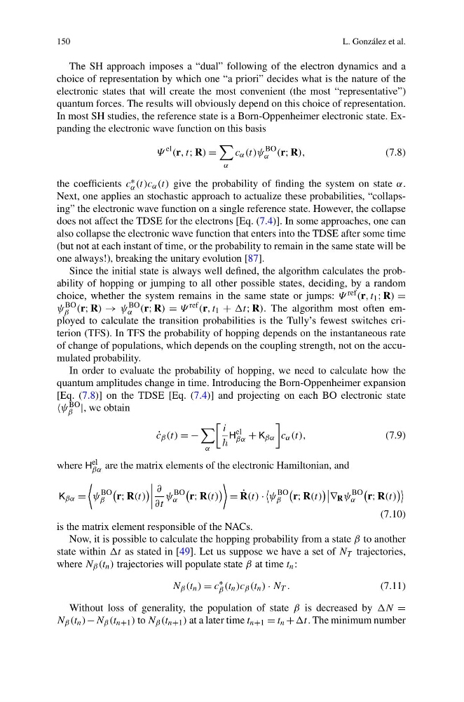
In most SH studies, the reference state is a Born-Oppenheimer electronic state. Expanding the electronic wave function on this basis
Ψ
el (r, t; R) =
α
c α (t)ψ
BO
α (r; R),
(7.8)
the coefficients c ∗
α (t)c α (t) give the probability of finding the system on state α.
Next, one applies an stochastic approach to actualize these probabilities, “collapsing” the electronic wave function on a single reference state. However, the collapse
does not affect the TDSE for the electrons [Eq. (7.4)]. In some approaches, one can
also collapse the electronic wave function that enters into the TDSE after some time
(but not at each instant of time, or the probability to remain in the same state will be
one always!), breaking the unitary evolution [87].
Since the initial state is always well defined, the algorithm calculates the probability of hopping or jumping to all other possible states, deciding, by a random
choice, whether the system remains in the same state or jumps: Ψ ref (r, t 1 ; R) =
ψ BO
β (r; R) → ψ BO
α (r; R) = Ψ ref (r, t 1 + t; R). The algorithm most often employed to calculate the transition probabilities is the Tully’s fewest switches criterion (TFS). In TFS the probability of hopping depends on the instantaneous rate
of change of populations, which depends on the coupling strength, not on the accumulated probability.
In order to evaluate the probability of hopping, we need to calculate how the
quantum amplitudes change in time. Introducing the Born-Oppenheimer expansion
[Eq. (7.8)] on the TDSE [Eq. (7.4)] and projecting on each BO electronic state
ψ BO
β |, we obtain
˙
c β (t) = −
α
i
H
el
βα + K βα
c α (t),
(7.9)
where H el
βα are the matrix elements of the electronic Hamiltonian, and
K βα =
ψ
BO
β
r; R(t)
∂
∂t
ψ
BO
α
r; R(t)
= ˙
R(t) ·
ψ
BO
β
r; R(t)
∇ R ψ
BO
α
r; R(t)
(7.10)
is the matrix element responsible of the NACs.
Now, it is possible to calculate the hopping probability from a state β to another
state within t as stated in [49]. Let us suppose we have a set of N T trajectories,
where N β (t n ) trajectories will populate state β at time t n :
N β (t n ) = c
∗
β (t n )c β (t n ) · N T .
(7.11)
Without loss of generality, the population of state β is decreased by N =
N β (t n )−N β (t n+1 ) to N β (t n+1 ) at a later time t n+1 = t n +t. The minimum number
L. González et al.
The SH approach imposes a “dual” following of the electron dynamics and a
choice of representation by which one “a priori” decides what is the nature of the
electronic states that will create the most convenient (the most “representative”)
quantum forces. The results will obviously depend on this choice of representation.
In most SH studies, the reference state is a Born-Oppenheimer electronic state. Expanding the electronic wave function on this basis
Ψ
el (r, t; R) =
α
c α (t)ψ
BO
α (r; R),
(7.8)
the coefficients c ∗
α (t)c α (t) give the probability of finding the system on state α.
Next, one applies an stochastic approach to actualize these probabilities, “collapsing” the electronic wave function on a single reference state. However, the collapse
does not affect the TDSE for the electrons [Eq. (7.4)]. In some approaches, one can
also collapse the electronic wave function that enters into the TDSE after some time
(but not at each instant of time, or the probability to remain in the same state will be
one always!), breaking the unitary evolution [87].
Since the initial state is always well defined, the algorithm calculates the probability of hopping or jumping to all other possible states, deciding, by a random
choice, whether the system remains in the same state or jumps: Ψ ref (r, t 1 ; R) =
ψ BO
β (r; R) → ψ BO
α (r; R) = Ψ ref (r, t 1 + t; R). The algorithm most often employed to calculate the transition probabilities is the Tully’s fewest switches criterion (TFS). In TFS the probability of hopping depends on the instantaneous rate
of change of populations, which depends on the coupling strength, not on the accumulated probability.
In order to evaluate the probability of hopping, we need to calculate how the
quantum amplitudes change in time. Introducing the Born-Oppenheimer expansion
[Eq. (7.8)] on the TDSE [Eq. (7.4)] and projecting on each BO electronic state
ψ BO
β |, we obtain
˙
c β (t) = −
α
i
H
el
βα + K βα
c α (t),
(7.9)
where H el
βα are the matrix elements of the electronic Hamiltonian, and
K βα =
ψ
BO
β
r; R(t)
∂
∂t
ψ
BO
α
r; R(t)
= ˙
R(t) ·
ψ
BO
β
r; R(t)
∇ R ψ
BO
α
r; R(t)
(7.10)
is the matrix element responsible of the NACs.
Now, it is possible to calculate the hopping probability from a state β to another
state within t as stated in [49]. Let us suppose we have a set of N T trajectories,
where N β (t n ) trajectories will populate state β at time t n :
N β (t n ) = c
∗
β (t n )c β (t n ) · N T .
(7.11)
Without loss of generality, the population of state β is decreased by N =
N β (t n )−N β (t n+1 ) to N β (t n+1 ) at a later time t n+1 = t n +t. The minimum number