

84
3 Electronic Excitation and Decay
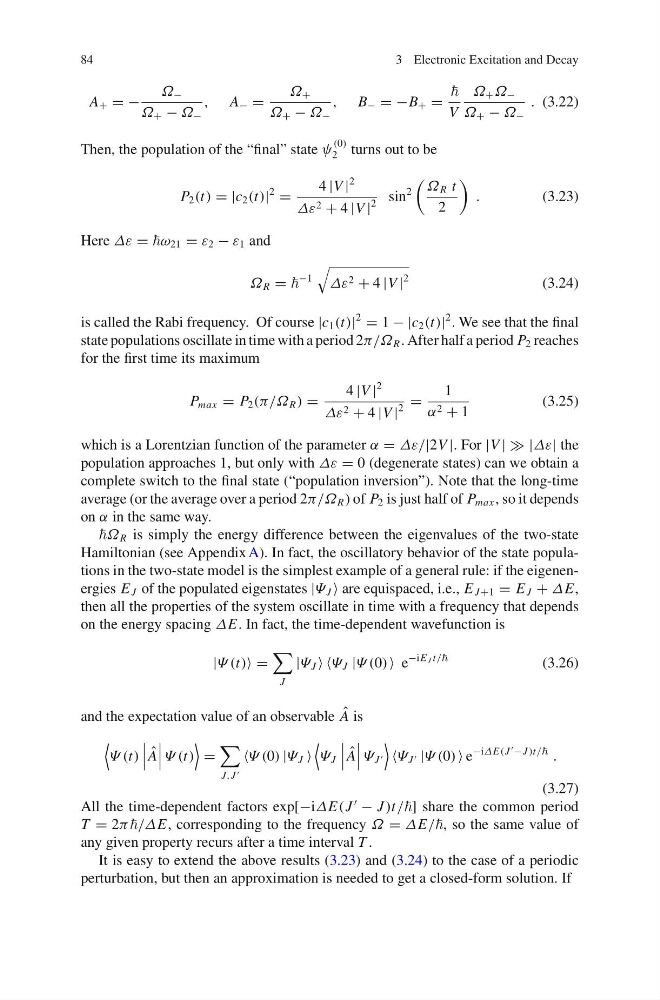
A + = −
Ω −
Ω + − Ω −
, A − =
Ω +
Ω + − Ω −
, B − = −B + =
V
Ω + Ω −
Ω + − Ω −
. (3.22)
Then, the population of the “final” state ψ
(0)
2 turns out to be
P 2 (t) = |c 2 (t)|
2
=
4 |V |
2
Δε 2 + 4 |V |
2
sin
2
Ω R t
2
.
(3.23)
Here Δε = ω 21 = ε 2 − ε 1 and
Ω R =
−1
Δε 2 + 4 |V |
2
(3.24)
is called the Rabi frequency. Of course |c 1 (t)|
2
= 1 − |c 2 (t)|
2 . We see that the final
state populations oscillate in time with a period 2π/Ω R . After half a period P 2 reaches
for the first time its maximum
P max = P 2 (π/Ω R ) =
4 |V |
2
Δε 2 + 4 |V |
2
=
1
α 2 + 1
(3.25)
which is a Lorentzian function of the parameter α = Δε/|2V |. For |V | | |Δε| the
population approaches 1, but only with Δε = 0 (degenerate states) can we obtain a
complete switch to the final state (“population inversion”). Note that the long-time
average (or the average over a period 2π/Ω R ) of P 2 is just half of P max , so it depends
on α in the same way.
Ω R is simply the energy difference between the eigenvalues of the two-state
Hamiltonian (see Appendix A). In fact, the oscillatory behavior of the state populations in the two-state model is the simplest example of a general rule: if the eigenenergies E J of the populated eigenstates |Ψ J are equispaced, i.e., E J +1 = E J + ΔE,
then all the properties of the system oscillate in time with a frequency that depends
on the energy spacing ΔE. In fact, the time-dependent wavefunction is
|Ψ (t) =
J
|Ψ J Ψ J |Ψ (0) e
−iE J t/
(3.26)
and the expectation value of an observable ˆ
A is
Ψ (t)
ˆ
A
Ψ (t)
=
J,J
Ψ (0) |Ψ J
Ψ J
ˆ
A
Ψ J
Ψ J |Ψ (0) e
−iΔE(J
−J )t/
.
(3.27)
All the time-dependent factors exp[−iΔE(J
− J )t/] share the common period
T = 2π /ΔE, corresponding to the frequency Ω = ΔE/, so the same value of
any given property recurs after a time interval T .
It is easy to extend the above results (3.23) and (3.24) to the case of a periodic
perturbation, but then an approximation is needed to get a closed-form solution. If
3 Electronic Excitation and Decay
A + = −
Ω −
Ω + − Ω −
, A − =
Ω +
Ω + − Ω −
, B − = −B + =
V
Ω + Ω −
Ω + − Ω −
. (3.22)
Then, the population of the “final” state ψ
(0)
2 turns out to be
P 2 (t) = |c 2 (t)|
2
=
4 |V |
2
Δε 2 + 4 |V |
2
sin
2
Ω R t
2
.
(3.23)
Here Δε = ω 21 = ε 2 − ε 1 and
Ω R =
−1
Δε 2 + 4 |V |
2
(3.24)
is called the Rabi frequency. Of course |c 1 (t)|
2
= 1 − |c 2 (t)|
2 . We see that the final
state populations oscillate in time with a period 2π/Ω R . After half a period P 2 reaches
for the first time its maximum
P max = P 2 (π/Ω R ) =
4 |V |
2
Δε 2 + 4 |V |
2
=
1
α 2 + 1
(3.25)
which is a Lorentzian function of the parameter α = Δε/|2V |. For |V | | |Δε| the
population approaches 1, but only with Δε = 0 (degenerate states) can we obtain a
complete switch to the final state (“population inversion”). Note that the long-time
average (or the average over a period 2π/Ω R ) of P 2 is just half of P max , so it depends
on α in the same way.
Ω R is simply the energy difference between the eigenvalues of the two-state
Hamiltonian (see Appendix A). In fact, the oscillatory behavior of the state populations in the two-state model is the simplest example of a general rule: if the eigenenergies E J of the populated eigenstates |Ψ J are equispaced, i.e., E J +1 = E J + ΔE,
then all the properties of the system oscillate in time with a frequency that depends
on the energy spacing ΔE. In fact, the time-dependent wavefunction is
|Ψ (t) =
J
|Ψ J Ψ J |Ψ (0) e
−iE J t/
(3.26)
and the expectation value of an observable ˆ
A is
Ψ (t)
ˆ
A
Ψ (t)
=
J,J
Ψ (0) |Ψ J
Ψ J
ˆ
A
Ψ J
Ψ J |Ψ (0) e
−iΔE(J
−J )t/
.
(3.27)
All the time-dependent factors exp[−iΔE(J
− J )t/] share the common period
T = 2π /ΔE, corresponding to the frequency Ω = ΔE/, so the same value of
any given property recurs after a time interval T .
It is easy to extend the above results (3.23) and (3.24) to the case of a periodic
perturbation, but then an approximation is needed to get a closed-form solution. If