

3.3 The Two-State Model: Rabi Oscillations
83
3.3 The Two-State Model: Rabi Oscillations
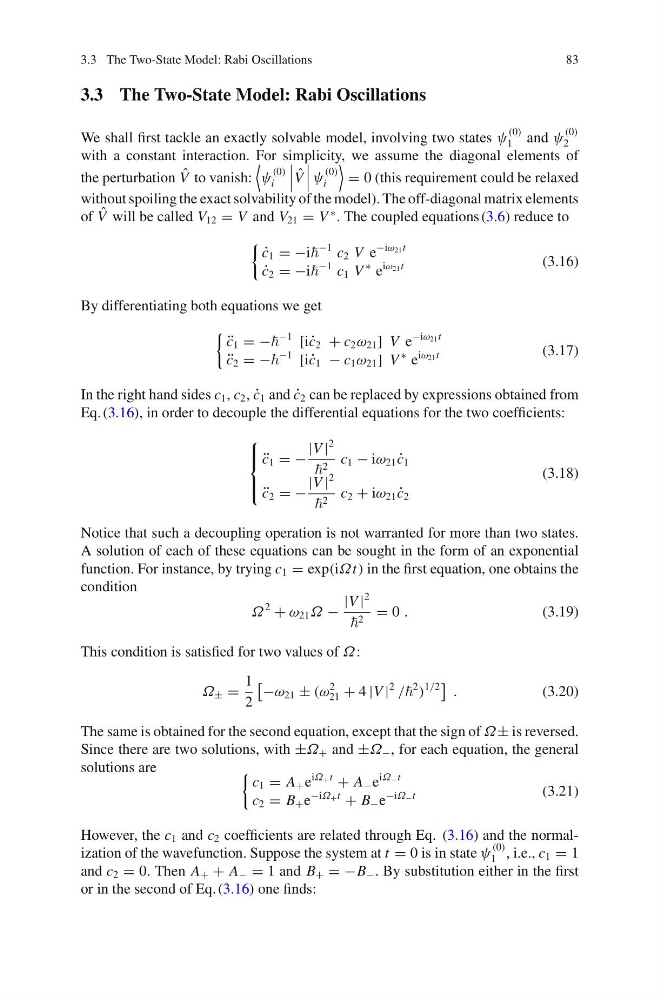
We shall first tackle an exactly solvable model, involving two states ψ
(0)
1 and ψ
(0)
2
with a constant interaction. For simplicity, we assume the diagonal elements of
the perturbation ˆ
V to vanish:
ψ
(0)
i
ˆ
V
ψ
(0)
i
= 0 (this requirement could be relaxed
without spoiling the exact solvability of the model). The off-diagonal matrix elements
of ˆ
V will be called V 12 = V and V 21 = V
∗ . The coupled equations (3.6) reduce to
˙
c 1 = −i
−1 c 2 V e
−iω 21 t
˙
c 2 = −i
−1 c 1 V
∗ e
iω 21 t
(3.16)
By differentiating both equations we get
¨
c 1 = −
−1 [i ˙
c 2 + c 2 ω 21 ] V e
−iω 21 t
¨
c 2 = −
−1 [i ˙
c 1 − c 1 ω 21 ] V
∗ e
iω 21 t
(3.17)
In the right hand sides c 1 , c 2 , ˙
c 1 and ˙
c 2 can be replaced by expressions obtained from
Eq. (3.16), in order to decouple the differential equations for the two coefficients:
⎧
⎪ ⎨
⎪ ⎩
¨
c 1 = −
|V |
2
2 c 1 − iω 21 ˙
c 1
¨
c 2 = −
|V |
2
2 c 2 + iω 21 ˙
c 2
(3.18)
Notice that such a decoupling operation is not warranted for more than two states.
A solution of each of these equations can be sought in the form of an exponential
function. For instance, by trying c 1 = exp(iΩt) in the first equation, one obtains the
condition
Ω
2
+ ω 21 Ω −
|V |
2
2 = 0 .
(3.19)
This condition is satisfied for two values of Ω:
Ω ± =
1
2
−ω 21 ± (ω
2
21 + 4 |V |
2
/
2
)
1/2
.
(3.20)
The same is obtained for the second equation, except that the sign of Ω± is reversed.
Since there are two solutions, with ±Ω + and ±Ω − , for each equation, the general
solutions are
c 1 = A + e
iΩ + t
+ A − e
iΩ − t
c 2 = B + e
−iΩ + t
+ B − e
−iΩ − t
(3.21)
However, the c 1 and c 2 coefficients are related through Eq. (3.16) and the normalization of the wavefunction. Suppose the system at t = 0 is in state ψ
(0)
1 , i.e., c 1 = 1
and c 2 = 0. Then A + + A − = 1 and B + = −B − . By substitution either in the first
or in the second of Eq. (3.16) one finds:
83
3.3 The Two-State Model: Rabi Oscillations
We shall first tackle an exactly solvable model, involving two states ψ
(0)
1 and ψ
(0)
2
with a constant interaction. For simplicity, we assume the diagonal elements of
the perturbation ˆ
V to vanish:
ψ
(0)
i
ˆ
V
ψ
(0)
i
= 0 (this requirement could be relaxed
without spoiling the exact solvability of the model). The off-diagonal matrix elements
of ˆ
V will be called V 12 = V and V 21 = V
∗ . The coupled equations (3.6) reduce to
˙
c 1 = −i
−1 c 2 V e
−iω 21 t
˙
c 2 = −i
−1 c 1 V
∗ e
iω 21 t
(3.16)
By differentiating both equations we get
¨
c 1 = −
−1 [i ˙
c 2 + c 2 ω 21 ] V e
−iω 21 t
¨
c 2 = −
−1 [i ˙
c 1 − c 1 ω 21 ] V
∗ e
iω 21 t
(3.17)
In the right hand sides c 1 , c 2 , ˙
c 1 and ˙
c 2 can be replaced by expressions obtained from
Eq. (3.16), in order to decouple the differential equations for the two coefficients:
⎧
⎪ ⎨
⎪ ⎩
¨
c 1 = −
|V |
2
2 c 1 − iω 21 ˙
c 1
¨
c 2 = −
|V |
2
2 c 2 + iω 21 ˙
c 2
(3.18)
Notice that such a decoupling operation is not warranted for more than two states.
A solution of each of these equations can be sought in the form of an exponential
function. For instance, by trying c 1 = exp(iΩt) in the first equation, one obtains the
condition
Ω
2
+ ω 21 Ω −
|V |
2
2 = 0 .
(3.19)
This condition is satisfied for two values of Ω:
Ω ± =
1
2
−ω 21 ± (ω
2
21 + 4 |V |
2
/
2
)
1/2
.
(3.20)
The same is obtained for the second equation, except that the sign of Ω± is reversed.
Since there are two solutions, with ±Ω + and ±Ω − , for each equation, the general
solutions are
c 1 = A + e
iΩ + t
+ A − e
iΩ − t
c 2 = B + e
−iΩ + t
+ B − e
−iΩ − t
(3.21)
However, the c 1 and c 2 coefficients are related through Eq. (3.16) and the normalization of the wavefunction. Suppose the system at t = 0 is in state ψ
(0)
1 , i.e., c 1 = 1
and c 2 = 0. Then A + + A − = 1 and B + = −B − . By substitution either in the first
or in the second of Eq. (3.16) one finds: