

2.4 The Electrostatic Approximation: Spin and Magnetic Couplings
47
is the one-electron spin–orbit Hamiltonian (l = r × p). However, it is clear from
the above that a correct account of the spin–orbit interaction would imply a full
relativistic approach, which is far beyond the aim of this book (see, e.g., Greiner’s
textbooks [9, 10]). In the following, we will limit ourselves to show some of the most
used spin–orbit Hamiltonians, giving just a brief comment about their derivation.
The relativistic quantum mechanical equation of motion for the free electron is
the Dirac equation, where the wavefunction has four components, as it can describe
an electron or a positron with spin ±1/2. In particular, positive energy solutions
of the Dirac equation represent electrons, while negative energy solutions represent
positrons. The four components of the wavefunction are coupled, nevertheless a
simplification of the Dirac equation can be obtained by applying a transformation
which reduces the coupling between electronic and positronic solutions, yielding a
two-component one-electron Hamiltonian, from which the spin–orbit interaction can
be extracted. However, such a transformation may be performed in many different
ways, and correspondingly different forms of the SO interaction are obtained. In
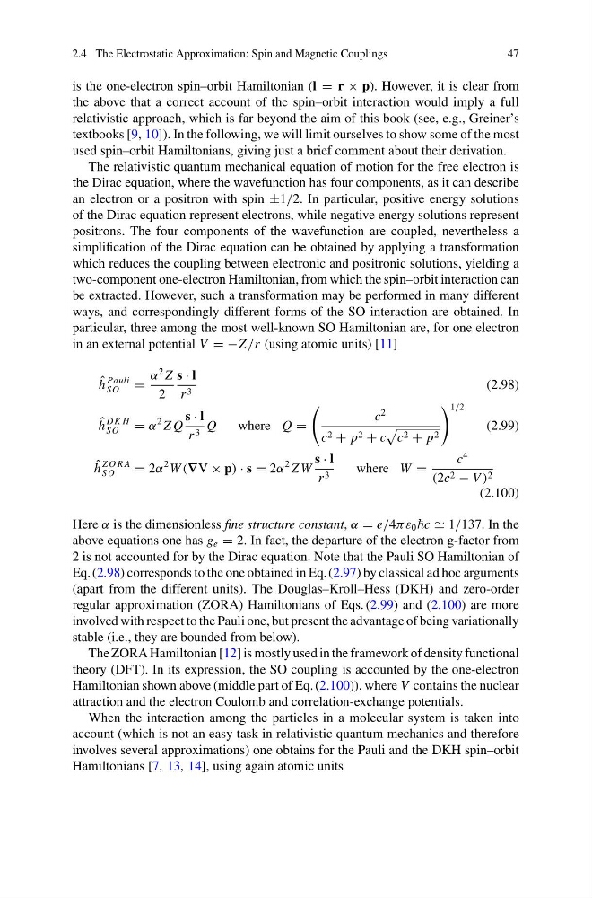
particular, three among the most well-known SO Hamiltonian are, for one electron
in an external potential V = −Z /r (using atomic units) [11]
ˆ
h
Pauli
SO
=
α
2 Z
2
s · l
r 3
(2.98)
ˆ
h
DK H
SO
= α
2 Z Q
s · l
r 3 Q
where Q =
c
2
c 2 + p 2 + c
c 2 + p 2
1/2
(2.99)
ˆ
h
Z O R A
SO
= 2α
2 W (∇V × p) · s = 2α
2 Z W
s · l
r 3
where W =
c
4
(2c 2 − V ) 2
(2.100)
Here α is the dimensionless fine structure constant, α = e/4πε 0 c 1/137. In the
above equations one has g e = 2. In fact, the departure of the electron g-factor from
2 is not accounted for by the Dirac equation. Note that the Pauli SO Hamiltonian of
Eq. (2.98) corresponds to the one obtained in Eq. (2.97) by classical ad hoc arguments
(apart from the different units). The Douglas–Kroll–Hess (DKH) and zero-order
regular approximation (ZORA) Hamiltonians of Eqs. (2.99) and (2.100) are more
involved with respect to the Pauli one, but present the advantage of being variationally
stable (i.e., they are bounded from below).
The ZORA Hamiltonian [12] is mostly used in the framework of density functional
theory (DFT). In its expression, the SO coupling is accounted by the one-electron
Hamiltonian shown above (middle part of Eq. (2.100)), where V contains the nuclear
attraction and the electron Coulomb and correlation-exchange potentials.
When the interaction among the particles in a molecular system is taken into
account (which is not an easy task in relativistic quantum mechanics and therefore
involves several approximations) one obtains for the Pauli and the DKH spin–orbit
Hamiltonians [7, 13, 14], using again atomic units
47
is the one-electron spin–orbit Hamiltonian (l = r × p). However, it is clear from
the above that a correct account of the spin–orbit interaction would imply a full
relativistic approach, which is far beyond the aim of this book (see, e.g., Greiner’s
textbooks [9, 10]). In the following, we will limit ourselves to show some of the most
used spin–orbit Hamiltonians, giving just a brief comment about their derivation.
The relativistic quantum mechanical equation of motion for the free electron is
the Dirac equation, where the wavefunction has four components, as it can describe
an electron or a positron with spin ±1/2. In particular, positive energy solutions
of the Dirac equation represent electrons, while negative energy solutions represent
positrons. The four components of the wavefunction are coupled, nevertheless a
simplification of the Dirac equation can be obtained by applying a transformation
which reduces the coupling between electronic and positronic solutions, yielding a
two-component one-electron Hamiltonian, from which the spin–orbit interaction can
be extracted. However, such a transformation may be performed in many different
ways, and correspondingly different forms of the SO interaction are obtained. In
particular, three among the most well-known SO Hamiltonian are, for one electron
in an external potential V = −Z /r (using atomic units) [11]
ˆ
h
Pauli
SO
=
α
2 Z
2
s · l
r 3
(2.98)
ˆ
h
DK H
SO
= α
2 Z Q
s · l
r 3 Q
where Q =
c
2
c 2 + p 2 + c
c 2 + p 2
1/2
(2.99)
ˆ
h
Z O R A
SO
= 2α
2 W (∇V × p) · s = 2α
2 Z W
s · l
r 3
where W =
c
4
(2c 2 − V ) 2
(2.100)
Here α is the dimensionless fine structure constant, α = e/4πε 0 c 1/137. In the
above equations one has g e = 2. In fact, the departure of the electron g-factor from
2 is not accounted for by the Dirac equation. Note that the Pauli SO Hamiltonian of
Eq. (2.98) corresponds to the one obtained in Eq. (2.97) by classical ad hoc arguments
(apart from the different units). The Douglas–Kroll–Hess (DKH) and zero-order
regular approximation (ZORA) Hamiltonians of Eqs. (2.99) and (2.100) are more
involved with respect to the Pauli one, but present the advantage of being variationally
stable (i.e., they are bounded from below).
The ZORA Hamiltonian [12] is mostly used in the framework of density functional
theory (DFT). In its expression, the SO coupling is accounted by the one-electron
Hamiltonian shown above (middle part of Eq. (2.100)), where V contains the nuclear
attraction and the electron Coulomb and correlation-exchange potentials.
When the interaction among the particles in a molecular system is taken into
account (which is not an easy task in relativistic quantum mechanics and therefore
involves several approximations) one obtains for the Pauli and the DKH spin–orbit
Hamiltonians [7, 13, 14], using again atomic units