

2.4 The Electrostatic Approximation: Spin and Magnetic Couplings
43
2.4 The Electrostatic Approximation: Spin and Magnetic
Couplings
In the electrostatic approximation we neglect the spin terms in the electronic Hamiltonian, which is written as (see Eq. (2.35))
ˆ
H el,SF = ˆ
T e + V el .
(2.79)
The total electronic spin ˆ
S =
N e
i ˆ
s i commutes with ˆ
H el,SF so that, in the electrostatic
approximation, the electronic wavefunctions ϕ k (x; R) can be chosen as eigenstates
of ˆ
S
2 and ˆ
S z
ˆ
S
2
ϕ k (x; R) =
2 S k (S k + 1)ϕ k (x; R)
(2.80)
ˆ
S z ϕ k (x; R) = M S k ϕ k (x; R)
(2.81)
where x collects the spin and space electronic degrees of freedom. For a given value
of S k , the projection M S k of the spin on a quantization axis has 2S k + 1 different
values, which correspond to the same energy.
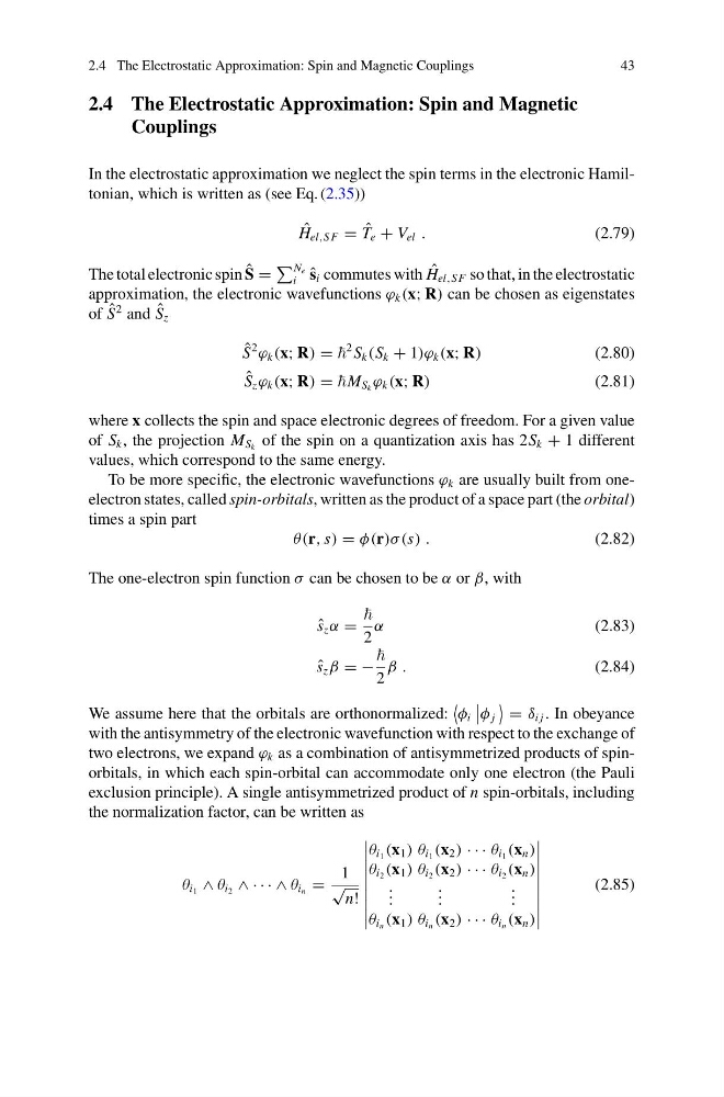
To be more specific, the electronic wavefunctions ϕ k are usually built from oneelectron states, called spin-orbitals, written as the product of a space part (the orbital)
times a spin part
θ(r, s) = φ(r)σ (s) .
(2.82)
The one-electron spin function σ can be chosen to be α or β, with
ˆ
s z α =
2
α
(2.83)
ˆ
s z β = −
2
β .
(2.84)
We assume here that the orbitals are orthonormalized:
φ i
φ j
= δ i j . In obeyance
with the antisymmetry of the electronic wavefunction with respect to the exchange of
two electrons, we expand ϕ k as a combination of antisymmetrized products of spinorbitals, in which each spin-orbital can accommodate only one electron (the Pauli
exclusion principle). A single antisymmetrized product of n spin-orbitals, including
the normalization factor, can be written as
θ i 1 ∧ θ i 2 ∧ · · · ∧ θ i n =
1
√
n!
θ i 1 (x 1 ) θ i 1 (x 2 ) · · · θ i 1 (x n )
θ i 2 (x 1 ) θ i 2 (x 2 ) · · · θ i 2 (x n )
. . .
. . .
. . .
θ i n (x 1 ) θ i n (x 2 ) · · · θ i n (x n )
(2.85)
43
2.4 The Electrostatic Approximation: Spin and Magnetic
Couplings
In the electrostatic approximation we neglect the spin terms in the electronic Hamiltonian, which is written as (see Eq. (2.35))
ˆ
H el,SF = ˆ
T e + V el .
(2.79)
The total electronic spin ˆ
S =
N e
i ˆ
s i commutes with ˆ
H el,SF so that, in the electrostatic
approximation, the electronic wavefunctions ϕ k (x; R) can be chosen as eigenstates
of ˆ
S
2 and ˆ
S z
ˆ
S
2
ϕ k (x; R) =
2 S k (S k + 1)ϕ k (x; R)
(2.80)
ˆ
S z ϕ k (x; R) = M S k ϕ k (x; R)
(2.81)
where x collects the spin and space electronic degrees of freedom. For a given value
of S k , the projection M S k of the spin on a quantization axis has 2S k + 1 different
values, which correspond to the same energy.
To be more specific, the electronic wavefunctions ϕ k are usually built from oneelectron states, called spin-orbitals, written as the product of a space part (the orbital)
times a spin part
θ(r, s) = φ(r)σ (s) .
(2.82)
The one-electron spin function σ can be chosen to be α or β, with
ˆ
s z α =
2
α
(2.83)
ˆ
s z β = −
2
β .
(2.84)
We assume here that the orbitals are orthonormalized:
φ i
φ j
= δ i j . In obeyance
with the antisymmetry of the electronic wavefunction with respect to the exchange of
two electrons, we expand ϕ k as a combination of antisymmetrized products of spinorbitals, in which each spin-orbital can accommodate only one electron (the Pauli
exclusion principle). A single antisymmetrized product of n spin-orbitals, including
the normalization factor, can be written as
θ i 1 ∧ θ i 2 ∧ · · · ∧ θ i n =
1
√
n!
θ i 1 (x 1 ) θ i 1 (x 2 ) · · · θ i 1 (x n )
θ i 2 (x 1 ) θ i 2 (x 2 ) · · · θ i 2 (x n )
. . .
. . .
. . .
θ i n (x 1 ) θ i n (x 2 ) · · · θ i n (x n )
(2.85)