

2.3 The Born–Oppenheimer Approximation and Its Breakdown …
39
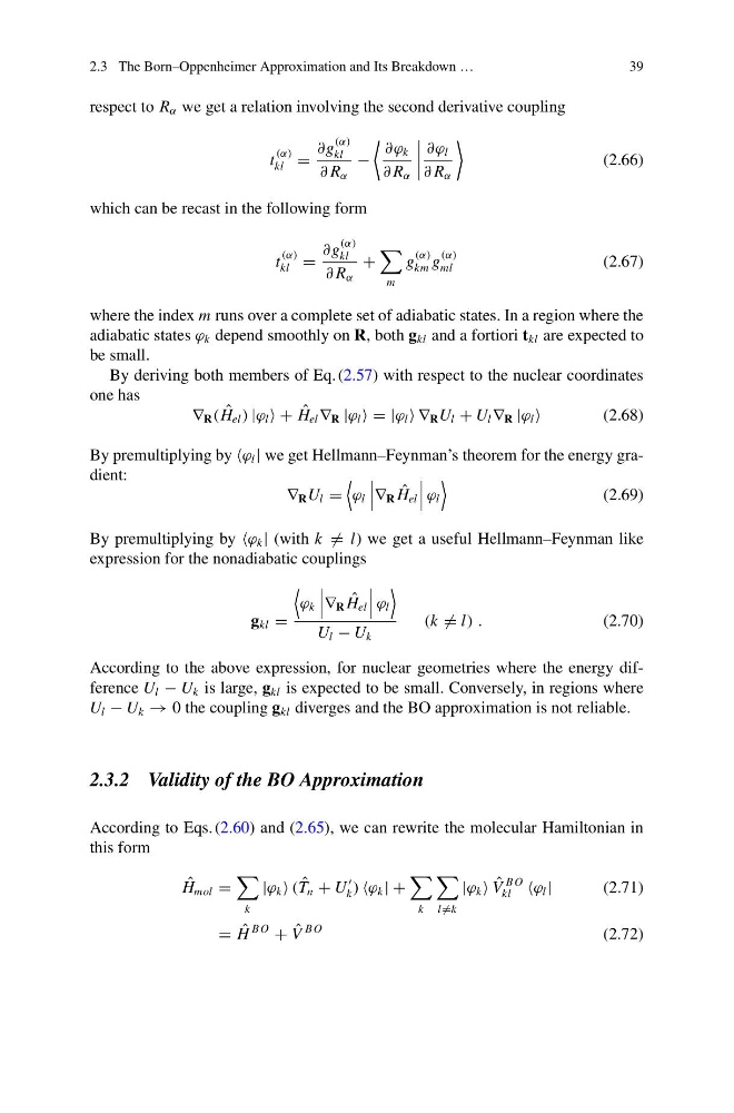
respect to R α we get a relation involving the second derivative coupling
t
(α)
kl =
∂g
(α)
kl
∂ R α
−
∂ϕ k
∂ R α
∂ϕ l
∂ R α
(2.66)
which can be recast in the following form
t
(α)
kl =
∂g
(α)
kl
∂ R α
+
m
g
(α)
km g
(α)
ml
(2.67)
where the index m runs over a complete set of adiabatic states. In a region where the
adiabatic states ϕ k depend smoothly on R, both g kl and a fortiori t kl are expected to
be small.
By deriving both members of Eq. (2.57) with respect to the nuclear coordinates
one has
∇ R ( ˆ
H el ) |ϕ l + ˆ
H el ∇ R |ϕ l = |ϕ l ∇ R U l + U l ∇ R |ϕ l
(2.68)
By premultiplying by ϕ l | we get Hellmann–Feynman’s theorem for the energy gradient:
∇ R U l =
ϕ l
∇R ˆ
H el
ϕ l
(2.69)
By premultiplying by ϕ k | (with k = l) we get a useful Hellmann–Feynman like
expression for the nonadiabatic couplings
g kl =
ϕ k
∇R ˆ
H el
ϕ l
U l − U k
(k = l) .
(2.70)
According to the above expression, for nuclear geometries where the energy difference U l − U k is large, g kl is expected to be small. Conversely, in regions where
U l − U k → 0 the coupling g kl diverges and the BO approximation is not reliable.
2.3.2 Validity of the BO Approximation
According to Eqs. (2.60) and (2.65), we can rewrite the molecular Hamiltonian in
this form
ˆ
H mol =
k
|ϕ k ( ˆ
T n + U
k ) ϕ k | +
k
l =k
|ϕ k ˆ
V
B O
kl ϕ l |
(2.71)
= ˆ
H
B O
+ ˆ
V
B O
(2.72)
39
respect to R α we get a relation involving the second derivative coupling
t
(α)
kl =
∂g
(α)
kl
∂ R α
−
∂ϕ k
∂ R α
∂ϕ l
∂ R α
(2.66)
which can be recast in the following form
t
(α)
kl =
∂g
(α)
kl
∂ R α
+
m
g
(α)
km g
(α)
ml
(2.67)
where the index m runs over a complete set of adiabatic states. In a region where the
adiabatic states ϕ k depend smoothly on R, both g kl and a fortiori t kl are expected to
be small.
By deriving both members of Eq. (2.57) with respect to the nuclear coordinates
one has
∇ R ( ˆ
H el ) |ϕ l + ˆ
H el ∇ R |ϕ l = |ϕ l ∇ R U l + U l ∇ R |ϕ l
(2.68)
By premultiplying by ϕ l | we get Hellmann–Feynman’s theorem for the energy gradient:
∇ R U l =
ϕ l
∇R ˆ
H el
ϕ l
(2.69)
By premultiplying by ϕ k | (with k = l) we get a useful Hellmann–Feynman like
expression for the nonadiabatic couplings
g kl =
ϕ k
∇R ˆ
H el
ϕ l
U l − U k
(k = l) .
(2.70)
According to the above expression, for nuclear geometries where the energy difference U l − U k is large, g kl is expected to be small. Conversely, in regions where
U l − U k → 0 the coupling g kl diverges and the BO approximation is not reliable.
2.3.2 Validity of the BO Approximation
According to Eqs. (2.60) and (2.65), we can rewrite the molecular Hamiltonian in
this form
ˆ
H mol =
k
|ϕ k ( ˆ
T n + U
k ) ϕ k | +
k
l =k
|ϕ k ˆ
V
B O
kl ϕ l |
(2.71)
= ˆ
H
B O
+ ˆ
V
B O
(2.72)