

30
2 Molecular States
2.1.2 Stationary States
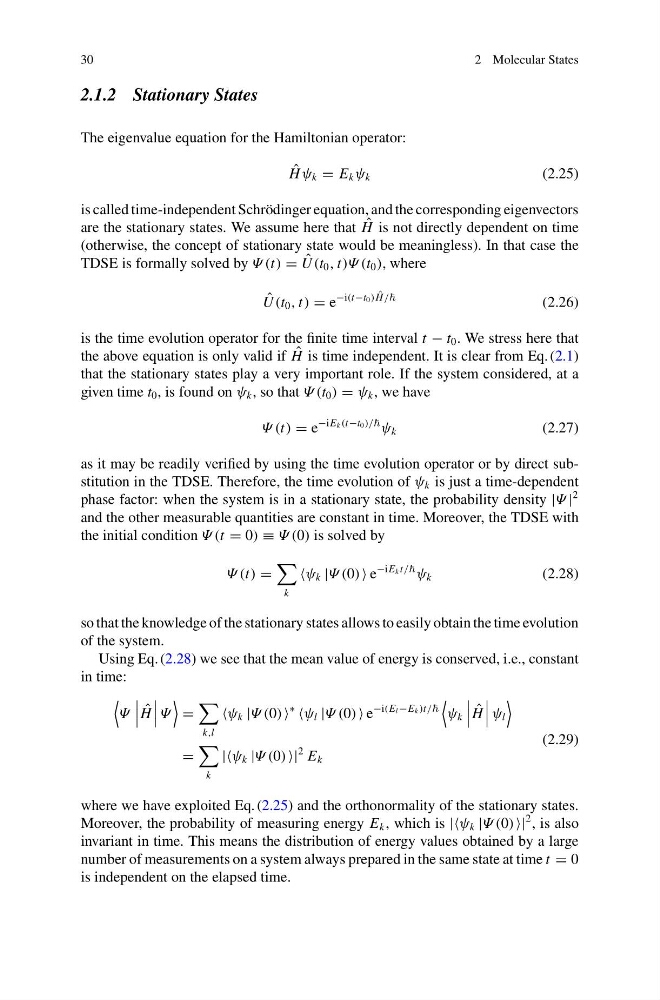
The eigenvalue equation for the Hamiltonian operator:
ˆ
H ψ k = E k ψ k
(2.25)
is called time-independent Schrödinger equation, and the corresponding eigenvectors
are the stationary states. We assume here that ˆ
H is not directly dependent on time
(otherwise, the concept of stationary state would be meaningless). In that case the
TDSE is formally solved by Ψ (t) = ˆ
U (t 0 , t)Ψ (t 0 ), where
ˆ
U (t 0 , t) = e
−i(t−t 0 ) ˆ
H /
(2.26)
is the time evolution operator for the finite time interval t − t 0 . We stress here that
the above equation is only valid if ˆ
H is time independent. It is clear from Eq. (2.1)
that the stationary states play a very important role. If the system considered, at a
given time t 0 , is found on ψ k , so that Ψ (t 0 ) = ψ k , we have
Ψ (t) = e
−iE k (t−t 0 )/
ψ k
(2.27)
as it may be readily verified by using the time evolution operator or by direct substitution in the TDSE. Therefore, the time evolution of ψ k is just a time-dependent
phase factor: when the system is in a stationary state, the probability density |Ψ |
2
and the other measurable quantities are constant in time. Moreover, the TDSE with
the initial condition Ψ (t = 0) ≡ Ψ (0) is solved by
Ψ (t) =
k
ψ k |Ψ (0) e
−iE k t/
ψ k
(2.28)
so that the knowledge of the stationary states allows to easily obtain the time evolution
of the system.
Using Eq. (2.28) we see that the mean value of energy is conserved, i.e., constant
in time:
Ψ
ˆ
H
Ψ
=
k,l
ψ k |Ψ (0)
∗
ψ l |Ψ (0) e
−i(E l −E k )t/
ψ k
ˆ
H
ψ l
=
k
||ψ k |Ψ (0) |
2 E k
(2.29)
where we have exploited Eq. (2.25) and the orthonormality of the stationary states.
Moreover, the probability of measuring energy E k , which is ||ψ k |Ψ (0) |
2 , is also
invariant in time. This means the distribution of energy values obtained by a large
number of measurements on a system always prepared in the same state at time t = 0
is independent on the elapsed time.
2 Molecular States
2.1.2 Stationary States
The eigenvalue equation for the Hamiltonian operator:
ˆ
H ψ k = E k ψ k
(2.25)
is called time-independent Schrödinger equation, and the corresponding eigenvectors
are the stationary states. We assume here that ˆ
H is not directly dependent on time
(otherwise, the concept of stationary state would be meaningless). In that case the
TDSE is formally solved by Ψ (t) = ˆ
U (t 0 , t)Ψ (t 0 ), where
ˆ
U (t 0 , t) = e
−i(t−t 0 ) ˆ
H /
(2.26)
is the time evolution operator for the finite time interval t − t 0 . We stress here that
the above equation is only valid if ˆ
H is time independent. It is clear from Eq. (2.1)
that the stationary states play a very important role. If the system considered, at a
given time t 0 , is found on ψ k , so that Ψ (t 0 ) = ψ k , we have
Ψ (t) = e
−iE k (t−t 0 )/
ψ k
(2.27)
as it may be readily verified by using the time evolution operator or by direct substitution in the TDSE. Therefore, the time evolution of ψ k is just a time-dependent
phase factor: when the system is in a stationary state, the probability density |Ψ |
2
and the other measurable quantities are constant in time. Moreover, the TDSE with
the initial condition Ψ (t = 0) ≡ Ψ (0) is solved by
Ψ (t) =
k
ψ k |Ψ (0) e
−iE k t/
ψ k
(2.28)
so that the knowledge of the stationary states allows to easily obtain the time evolution
of the system.
Using Eq. (2.28) we see that the mean value of energy is conserved, i.e., constant
in time:
Ψ
ˆ
H
Ψ
=
k,l
ψ k |Ψ (0)
∗
ψ l |Ψ (0) e
−i(E l −E k )t/
ψ k
ˆ
H
ψ l
=
k
||ψ k |Ψ (0) |
2 E k
(2.29)
where we have exploited Eq. (2.25) and the orthonormality of the stationary states.
Moreover, the probability of measuring energy E k , which is ||ψ k |Ψ (0) |
2 , is also
invariant in time. This means the distribution of energy values obtained by a large
number of measurements on a system always prepared in the same state at time t = 0
is independent on the elapsed time.