

2.1 The Time-Dependent Schrödinger Equation
29
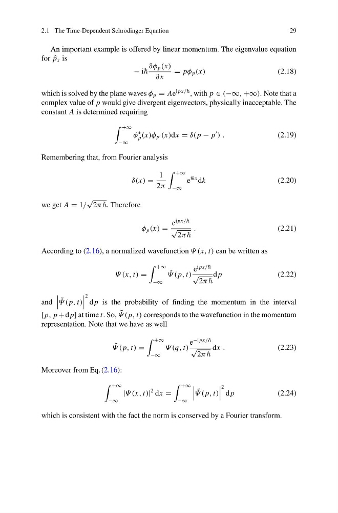
An important example is offered by linear momentum. The eigenvalue equation
for ˆ
p x is
− i
∂φ p (x)
∂ x
= pφ p (x)
(2.18)
which is solved by the plane waves φ p = Ae
i px/ , with p ∈ (−∞, +∞). Note that a
complex value of p would give divergent eigenvectors, physically inacceptable. The
constant A is determined requiring
+∞
−∞
φ
∗
p (x)φ p (x)dx = δ( p − p
) .
(2.19)
Remembering that, from Fourier analysis
δ(x) =
1
2π
+∞
−∞
e
ikx dk
(2.20)
we get A = 1/
√
2π . Therefore
φ p (x) =
e
i px/
√
2π
.
(2.21)
According to (2.16), a normalized wavefunction Ψ (x, t) can be written as
Ψ (x, t) =
+∞
−∞
˜
Ψ (p, t)
e
i px/
√
2π
d p
(2.22)
and
˜
Ψ (p, t)
2
d p is the probability of finding the momentum in the interval
[ p, p + d p] at time t. So, ˜
Ψ (p, t) corresponds to the wavefunction in the momentum
representation. Note that we have as well
˜
Ψ (p, t) =
+∞
−∞
Ψ (q, t)
e
−i px/
√
2π
dx .
(2.23)
Moreover from Eq. (2.16):
+∞
−∞
|Ψ (x, t)|
2 dx =
+∞
−∞
˜
Ψ (p, t)
2
d p
(2.24)
which is consistent with the fact the norm is conserved by a Fourier transform.
29
An important example is offered by linear momentum. The eigenvalue equation
for ˆ
p x is
− i
∂φ p (x)
∂ x
= pφ p (x)
(2.18)
which is solved by the plane waves φ p = Ae
i px/ , with p ∈ (−∞, +∞). Note that a
complex value of p would give divergent eigenvectors, physically inacceptable. The
constant A is determined requiring
+∞
−∞
φ
∗
p (x)φ p (x)dx = δ( p − p
) .
(2.19)
Remembering that, from Fourier analysis
δ(x) =
1
2π
+∞
−∞
e
ikx dk
(2.20)
we get A = 1/
√
2π . Therefore
φ p (x) =
e
i px/
√
2π
.
(2.21)
According to (2.16), a normalized wavefunction Ψ (x, t) can be written as
Ψ (x, t) =
+∞
−∞
˜
Ψ (p, t)
e
i px/
√
2π
d p
(2.22)
and
˜
Ψ (p, t)
2
d p is the probability of finding the momentum in the interval
[ p, p + d p] at time t. So, ˜
Ψ (p, t) corresponds to the wavefunction in the momentum
representation. Note that we have as well
˜
Ψ (p, t) =
+∞
−∞
Ψ (q, t)
e
−i px/
√
2π
dx .
(2.23)
Moreover from Eq. (2.16):
+∞
−∞
|Ψ (x, t)|
2 dx =
+∞
−∞
˜
Ψ (p, t)
2
d p
(2.24)
which is consistent with the fact the norm is conserved by a Fourier transform.