

196
6 Charge and Energy Transfer Processes
Y,LL
X,KK
R
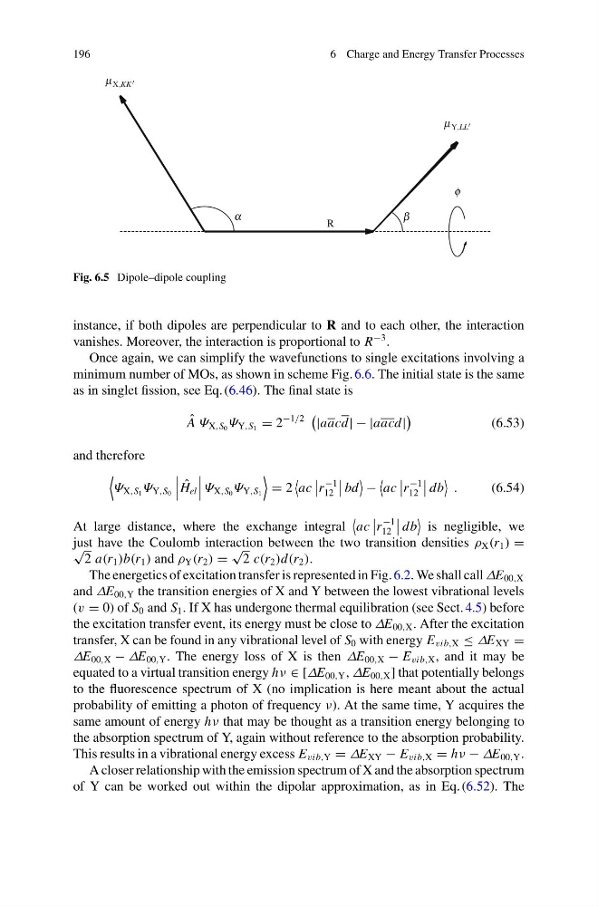
Fig. 6.5 Dipole–dipole coupling
instance, if both dipoles are perpendicular to R and to each other, the interaction
vanishes. Moreover, the interaction is proportional to R
−3 .
Once again, we can simplify the wavefunctions to single excitations involving a
minimum number of MOs, as shown in scheme Fig. 6.6. The initial state is the same
as in singlet fission, see Eq. (6.46). The final state is
ˆ
A Ψ X,S 0 Ψ Y,S 1 = 2
−1/2
|aacd| − |aacd|
(6.53)
and therefore
Ψ X,S 1 Ψ Y,S 0
ˆ
H el
Ψ X,S 0 Ψ Y,S 1
= 2
ac
r
−1
12
bd
−
ac
r
−1
12
db
.
(6.54)
At large distance, where the exchange integral
ac
r
−1
12
db
is negligible, we
just have the Coulomb interaction between the two transition densities ρ X (r 1 ) =
√
2 a(r 1 )b(r 1 ) and ρ Y (r 2 ) =
√
2 c(r 2 )d(r 2 ).
The energetics of excitation transfer is represented in Fig. 6.2. We shall call ΔE 00,X
and ΔE 00,Y the transition energies of X and Y between the lowest vibrational levels
(v = 0) of S 0 and S 1 . If X has undergone thermal equilibration (see Sect. 4.5) before
the excitation transfer event, its energy must be close to ΔE 00,X . After the excitation
transfer, X can be found in any vibrational level of S 0 with energy E vib,X ≤ ΔE XY =
ΔE 00,X − ΔE 00,Y . The energy loss of X is then ΔE 00,X − E vib,X , and it may be
equated to a virtual transition energy hν ∈ [ΔE 00,Y , ΔE 00,X ] that potentially belongs
to the fluorescence spectrum of X (no implication is here meant about the actual
probability of emitting a photon of frequency ν). At the same time, Y acquires the
same amount of energy hν that may be thought as a transition energy belonging to
the absorption spectrum of Y, again without reference to the absorption probability.
This results in a vibrational energy excess E vib,Y = ΔE XY − E vib,X = hν − ΔE 00,Y .
A closer relationship with the emission spectrum of X and the absorption spectrum
of Y can be worked out within the dipolar approximation, as in Eq. (6.52). The
6 Charge and Energy Transfer Processes
Y,LL
X,KK
R
Fig. 6.5 Dipole–dipole coupling
instance, if both dipoles are perpendicular to R and to each other, the interaction
vanishes. Moreover, the interaction is proportional to R
−3 .
Once again, we can simplify the wavefunctions to single excitations involving a
minimum number of MOs, as shown in scheme Fig. 6.6. The initial state is the same
as in singlet fission, see Eq. (6.46). The final state is
ˆ
A Ψ X,S 0 Ψ Y,S 1 = 2
−1/2
|aacd| − |aacd|
(6.53)
and therefore
Ψ X,S 1 Ψ Y,S 0
ˆ
H el
Ψ X,S 0 Ψ Y,S 1
= 2
ac
r
−1
12
bd
−
ac
r
−1
12
db
.
(6.54)
At large distance, where the exchange integral
ac
r
−1
12
db
is negligible, we
just have the Coulomb interaction between the two transition densities ρ X (r 1 ) =
√
2 a(r 1 )b(r 1 ) and ρ Y (r 2 ) =
√
2 c(r 2 )d(r 2 ).
The energetics of excitation transfer is represented in Fig. 6.2. We shall call ΔE 00,X
and ΔE 00,Y the transition energies of X and Y between the lowest vibrational levels
(v = 0) of S 0 and S 1 . If X has undergone thermal equilibration (see Sect. 4.5) before
the excitation transfer event, its energy must be close to ΔE 00,X . After the excitation
transfer, X can be found in any vibrational level of S 0 with energy E vib,X ≤ ΔE XY =
ΔE 00,X − ΔE 00,Y . The energy loss of X is then ΔE 00,X − E vib,X , and it may be
equated to a virtual transition energy hν ∈ [ΔE 00,Y , ΔE 00,X ] that potentially belongs
to the fluorescence spectrum of X (no implication is here meant about the actual
probability of emitting a photon of frequency ν). At the same time, Y acquires the
same amount of energy hν that may be thought as a transition energy belonging to
the absorption spectrum of Y, again without reference to the absorption probability.
This results in a vibrational energy excess E vib,Y = ΔE XY − E vib,X = hν − ΔE 00,Y .
A closer relationship with the emission spectrum of X and the absorption spectrum
of Y can be worked out within the dipolar approximation, as in Eq. (6.52). The