

6.4 Localized Excitations and Energy Transfer Mechanisms
197
-
d
c
Y, S 1
b
a
X, S 0
d
c
Y, S 0
-
b
a
X, S 1
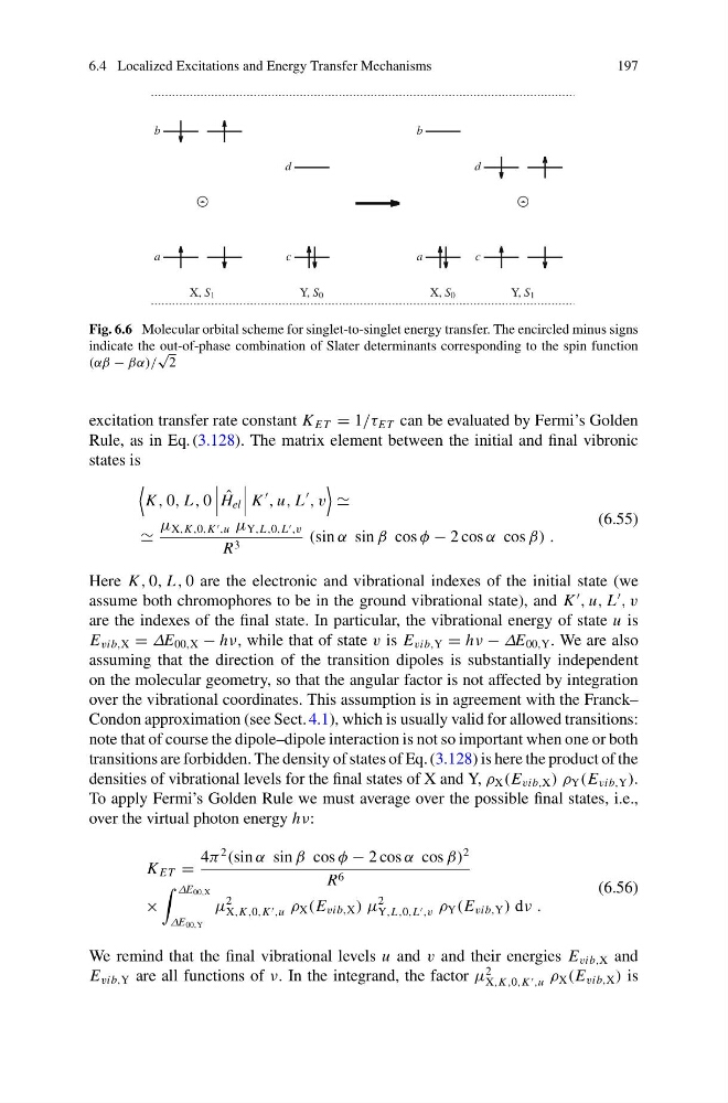
Fig. 6.6 Molecular orbital scheme for singlet-to-singlet energy transfer. The encircled minus signs
indicate the out-of-phase combination of Slater determinants corresponding to the spin function
(αβ − βα)/
√
2
excitation transfer rate constant K ET = 1/τ ET can be evaluated by Fermi’s Golden
Rule, as in Eq. (3.128). The matrix element between the initial and final vibronic
states is
K , 0, L , 0
ˆ
H el
K
, u, L
, v
μ X,K ,0,K ,u μ Y,L ,0,L ,v
R 3
(sin α sin β cos φ − 2 cos α cos β) .
(6.55)
Here K , 0, L , 0 are the electronic and vibrational indexes of the initial state (we
assume both chromophores to be in the ground vibrational state), and K
, u, L
, v
are the indexes of the final state. In particular, the vibrational energy of state u is
E vib,X = ΔE 00,X − hν, while that of state v is E vib,Y = hν − ΔE 00,Y . We are also
assuming that the direction of the transition dipoles is substantially independent
on the molecular geometry, so that the angular factor is not affected by integration
over the vibrational coordinates. This assumption is in agreement with the Franck–
Condon approximation (see Sect. 4.1), which is usually valid for allowed transitions:
note that of course the dipole–dipole interaction is not so important when one or both
transitions are forbidden. The density of states of Eq. (3.128) is here the product of the
densities of vibrational levels for the final states of X and Y, ρ X (E vib,X ) ρ Y (E vib,Y ).
To apply Fermi’s Golden Rule we must average over the possible final states, i.e.,
over the virtual photon energy hν:
K ET =
4π
2
(sin α sin β cos φ − 2 cos α cos β)
2
R 6
×
ΔE 00,X
ΔE 00,Y
μ
2
X,K ,0,K ,u ρ X (E vib,X ) μ
2
Y,L ,0,L ,v ρ Y (E vib,Y ) dν .
(6.56)
We remind that the final vibrational levels u and v and their energies E vib,X and
E vib,Y are all functions of ν. In the integrand, the factor μ
2
X,K ,0,K ,u ρ X (E vib,X ) is
197
-
d
c
Y, S 1
b
a
X, S 0
d
c
Y, S 0
-
b
a
X, S 1
Fig. 6.6 Molecular orbital scheme for singlet-to-singlet energy transfer. The encircled minus signs
indicate the out-of-phase combination of Slater determinants corresponding to the spin function
(αβ − βα)/
√
2
excitation transfer rate constant K ET = 1/τ ET can be evaluated by Fermi’s Golden
Rule, as in Eq. (3.128). The matrix element between the initial and final vibronic
states is
K , 0, L , 0
ˆ
H el
K
, u, L
, v
μ X,K ,0,K ,u μ Y,L ,0,L ,v
R 3
(sin α sin β cos φ − 2 cos α cos β) .
(6.55)
Here K , 0, L , 0 are the electronic and vibrational indexes of the initial state (we
assume both chromophores to be in the ground vibrational state), and K
, u, L
, v
are the indexes of the final state. In particular, the vibrational energy of state u is
E vib,X = ΔE 00,X − hν, while that of state v is E vib,Y = hν − ΔE 00,Y . We are also
assuming that the direction of the transition dipoles is substantially independent
on the molecular geometry, so that the angular factor is not affected by integration
over the vibrational coordinates. This assumption is in agreement with the Franck–
Condon approximation (see Sect. 4.1), which is usually valid for allowed transitions:
note that of course the dipole–dipole interaction is not so important when one or both
transitions are forbidden. The density of states of Eq. (3.128) is here the product of the
densities of vibrational levels for the final states of X and Y, ρ X (E vib,X ) ρ Y (E vib,Y ).
To apply Fermi’s Golden Rule we must average over the possible final states, i.e.,
over the virtual photon energy hν:
K ET =
4π
2
(sin α sin β cos φ − 2 cos α cos β)
2
R 6
×
ΔE 00,X
ΔE 00,Y
μ
2
X,K ,0,K ,u ρ X (E vib,X ) μ
2
Y,L ,0,L ,v ρ Y (E vib,Y ) dν .
(6.56)
We remind that the final vibrational levels u and v and their energies E vib,X and
E vib,Y are all functions of ν. In the integrand, the factor μ
2
X,K ,0,K ,u ρ X (E vib,X ) is