

5.5 Computational Note: Methods for Nonadiabatic Dynamics
173
˙
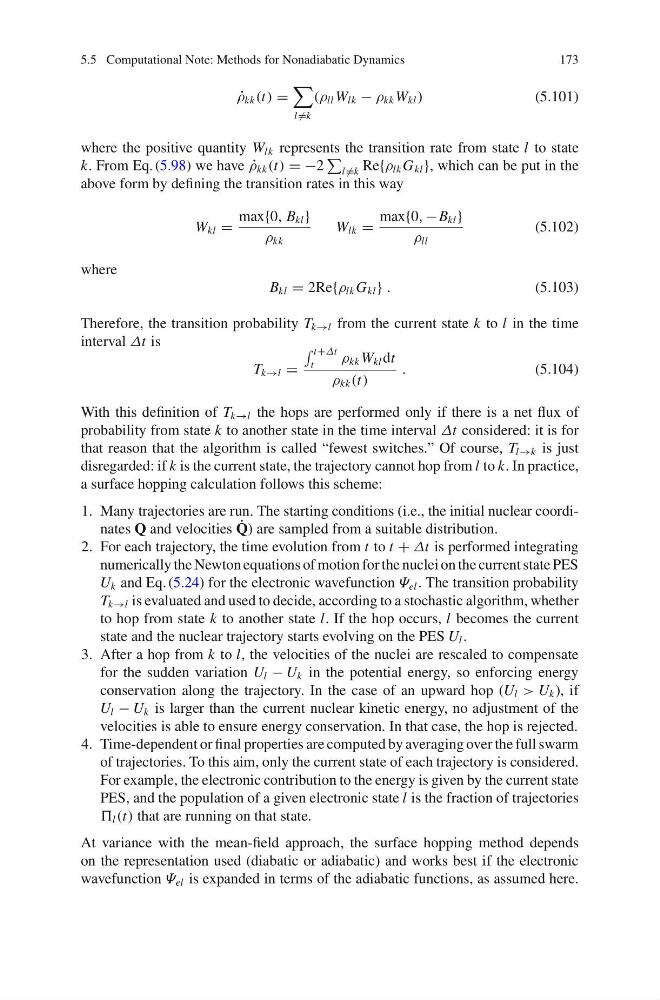
ρ kk (t) =
l =k
(ρ ll W lk − ρ kk W kl )
(5.101)
where the positive quantity W lk represents the transition rate from state l to state
k. From Eq. (5.98) we have ˙
ρ kk (t) = −2
l =k Re{ρ lk G kl }, which can be put in the
above form by defining the transition rates in this way
W kl =
max{0, B kl }
ρ kk
W lk =
max{0, −B kl }
ρ ll
(5.102)
where
B kl = 2Re{ρ lk G kl } .
(5.103)
Therefore, the transition probability T k→l from the current state k to l in the time
interval Δt is
T k→l =
t+Δt
t
ρ kk W kl dt
ρ kk (t)
.
(5.104)
With this definition of T k→l the hops are performed only if there is a net flux of
probability from state k to another state in the time interval Δt considered: it is for
that reason that the algorithm is called “fewest switches.” Of course, T l→k is just
disregarded: if k is the current state, the trajectory cannot hop from l to k. In practice,
a surface hopping calculation follows this scheme:
1. Many trajectories are run. The starting conditions (i.e., the initial nuclear coordinates Q and velocities ˙
Q) are sampled from a suitable distribution.
2. For each trajectory, the time evolution from t to t + Δt is performed integrating
numerically the Newton equations of motion for the nuclei on the current state PES
U k and Eq. (5.24) for the electronic wavefunction Ψ el . The transition probability
T k→l is evaluated and used to decide, according to a stochastic algorithm, whether
to hop from state k to another state l. If the hop occurs, l becomes the current
state and the nuclear trajectory starts evolving on the PES U l .
3. After a hop from k to l, the velocities of the nuclei are rescaled to compensate
for the sudden variation U l − U k in the potential energy, so enforcing energy
conservation along the trajectory. In the case of an upward hop (U l > U k ), if
U l − U k is larger than the current nuclear kinetic energy, no adjustment of the
velocities is able to ensure energy conservation. In that case, the hop is rejected.
4. Time-dependent or final properties are computed by averaging over the full swarm
of trajectories. To this aim, only the current state of each trajectory is considered.
For example, the electronic contribution to the energy is given by the current state
PES, and the population of a given electronic state l is the fraction of trajectories
l (t) that are running on that state.
At variance with the mean-field approach, the surface hopping method depends
on the representation used (diabatic or adiabatic) and works best if the electronic
wavefunction Ψ el is expanded in terms of the adiabatic functions, as assumed here.
173
˙
ρ kk (t) =
l =k
(ρ ll W lk − ρ kk W kl )
(5.101)
where the positive quantity W lk represents the transition rate from state l to state
k. From Eq. (5.98) we have ˙
ρ kk (t) = −2
l =k Re{ρ lk G kl }, which can be put in the
above form by defining the transition rates in this way
W kl =
max{0, B kl }
ρ kk
W lk =
max{0, −B kl }
ρ ll
(5.102)
where
B kl = 2Re{ρ lk G kl } .
(5.103)
Therefore, the transition probability T k→l from the current state k to l in the time
interval Δt is
T k→l =
t+Δt
t
ρ kk W kl dt
ρ kk (t)
.
(5.104)
With this definition of T k→l the hops are performed only if there is a net flux of
probability from state k to another state in the time interval Δt considered: it is for
that reason that the algorithm is called “fewest switches.” Of course, T l→k is just
disregarded: if k is the current state, the trajectory cannot hop from l to k. In practice,
a surface hopping calculation follows this scheme:
1. Many trajectories are run. The starting conditions (i.e., the initial nuclear coordinates Q and velocities ˙
Q) are sampled from a suitable distribution.
2. For each trajectory, the time evolution from t to t + Δt is performed integrating
numerically the Newton equations of motion for the nuclei on the current state PES
U k and Eq. (5.24) for the electronic wavefunction Ψ el . The transition probability
T k→l is evaluated and used to decide, according to a stochastic algorithm, whether
to hop from state k to another state l. If the hop occurs, l becomes the current
state and the nuclear trajectory starts evolving on the PES U l .
3. After a hop from k to l, the velocities of the nuclei are rescaled to compensate
for the sudden variation U l − U k in the potential energy, so enforcing energy
conservation along the trajectory. In the case of an upward hop (U l > U k ), if
U l − U k is larger than the current nuclear kinetic energy, no adjustment of the
velocities is able to ensure energy conservation. In that case, the hop is rejected.
4. Time-dependent or final properties are computed by averaging over the full swarm
of trajectories. To this aim, only the current state of each trajectory is considered.
For example, the electronic contribution to the energy is given by the current state
PES, and the population of a given electronic state l is the fraction of trajectories
l (t) that are running on that state.
At variance with the mean-field approach, the surface hopping method depends
on the representation used (diabatic or adiabatic) and works best if the electronic
wavefunction Ψ el is expanded in terms of the adiabatic functions, as assumed here.