

5.2 Diabatic States
145
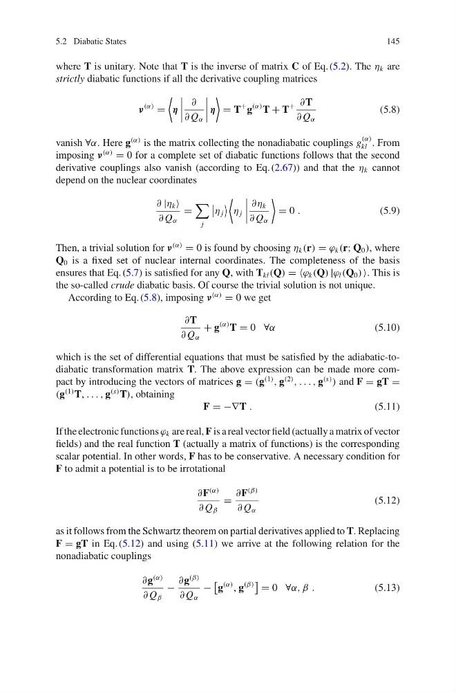
where T is unitary. Note that T is the inverse of matrix C of Eq. (5.2). The η k are
strictly diabatic functions if all the derivative coupling matrices
ν
(α)
=
η
∂
∂ Q α
η
= T
+ g
(α) T + T
+ ∂T
∂ Q α
(5.8)
vanish ∀α. Here g
(α) is the matrix collecting the nonadiabatic couplings g
(α)
kl . From
imposing ν
(α)
= 0 for a complete set of diabatic functions follows that the second
derivative couplings also vanish (according to Eq. (2.67)) and that the η k cannot
depend on the nuclear coordinates
∂ |η k
∂ Q α
=
j
η j
η j
∂η k
∂ Q α
= 0 .
(5.9)
Then, a trivial solution for ν
(α)
= 0 is found by choosing η k (r) = ϕ k (r; Q 0 ), where
Q 0 is a fixed set of nuclear internal coordinates. The completeness of the basis
ensures that Eq. (5.7) is satisfied for any Q, with T kl (Q) = ϕ k (Q) |ϕ l (Q 0 ) . This is
the so-called crude diabatic basis. Of course the trivial solution is not unique.
According to Eq. (5.8), imposing ν
(α)
= 0 we get
∂T
∂ Q α
+ g
(α) T = 0 ∀α
(5.10)
which is the set of differential equations that must be satisfied by the adiabatic-todiabatic transformation matrix T. The above expression can be made more compact by introducing the vectors of matrices g = (g
(1)
, g
(2)
, . . . , g
(s)
) and F = gT =
(g
(1) T, . . . , g
(s) T), obtaining
F = −∇T .
(5.11)
If the electronic functions ϕ k are real, F is a real vector field (actually a matrix of vector
fields) and the real function T (actually a matrix of functions) is the corresponding
scalar potential. In other words, F has to be conservative. A necessary condition for
F to admit a potential is to be irrotational
∂F
(α)
∂ Q β
=
∂F
(β)
∂ Q α
(5.12)
as it follows from the Schwartz theorem on partial derivatives applied to T. Replacing
F = gT in Eq. (5.12) and using (5.11) we arrive at the following relation for the
nonadiabatic couplings
∂g
(α)
∂ Q β
−
∂g
(β)
∂ Q α
−
g
(α)
, g
(β)
= 0 ∀α, β .
(5.13)
145
where T is unitary. Note that T is the inverse of matrix C of Eq. (5.2). The η k are
strictly diabatic functions if all the derivative coupling matrices
ν
(α)
=
η
∂
∂ Q α
η
= T
+ g
(α) T + T
+ ∂T
∂ Q α
(5.8)
vanish ∀α. Here g
(α) is the matrix collecting the nonadiabatic couplings g
(α)
kl . From
imposing ν
(α)
= 0 for a complete set of diabatic functions follows that the second
derivative couplings also vanish (according to Eq. (2.67)) and that the η k cannot
depend on the nuclear coordinates
∂ |η k
∂ Q α
=
j
η j
η j
∂η k
∂ Q α
= 0 .
(5.9)
Then, a trivial solution for ν
(α)
= 0 is found by choosing η k (r) = ϕ k (r; Q 0 ), where
Q 0 is a fixed set of nuclear internal coordinates. The completeness of the basis
ensures that Eq. (5.7) is satisfied for any Q, with T kl (Q) = ϕ k (Q) |ϕ l (Q 0 ) . This is
the so-called crude diabatic basis. Of course the trivial solution is not unique.
According to Eq. (5.8), imposing ν
(α)
= 0 we get
∂T
∂ Q α
+ g
(α) T = 0 ∀α
(5.10)
which is the set of differential equations that must be satisfied by the adiabatic-todiabatic transformation matrix T. The above expression can be made more compact by introducing the vectors of matrices g = (g
(1)
, g
(2)
, . . . , g
(s)
) and F = gT =
(g
(1) T, . . . , g
(s) T), obtaining
F = −∇T .
(5.11)
If the electronic functions ϕ k are real, F is a real vector field (actually a matrix of vector
fields) and the real function T (actually a matrix of functions) is the corresponding
scalar potential. In other words, F has to be conservative. A necessary condition for
F to admit a potential is to be irrotational
∂F
(α)
∂ Q β
=
∂F
(β)
∂ Q α
(5.12)
as it follows from the Schwartz theorem on partial derivatives applied to T. Replacing
F = gT in Eq. (5.12) and using (5.11) we arrive at the following relation for the
nonadiabatic couplings
∂g
(α)
∂ Q β
−
∂g
(β)
∂ Q α
−
g
(α)
, g
(β)
= 0 ∀α, β .
(5.13)