

146
5 Fast Nonadiabatic Dynamics
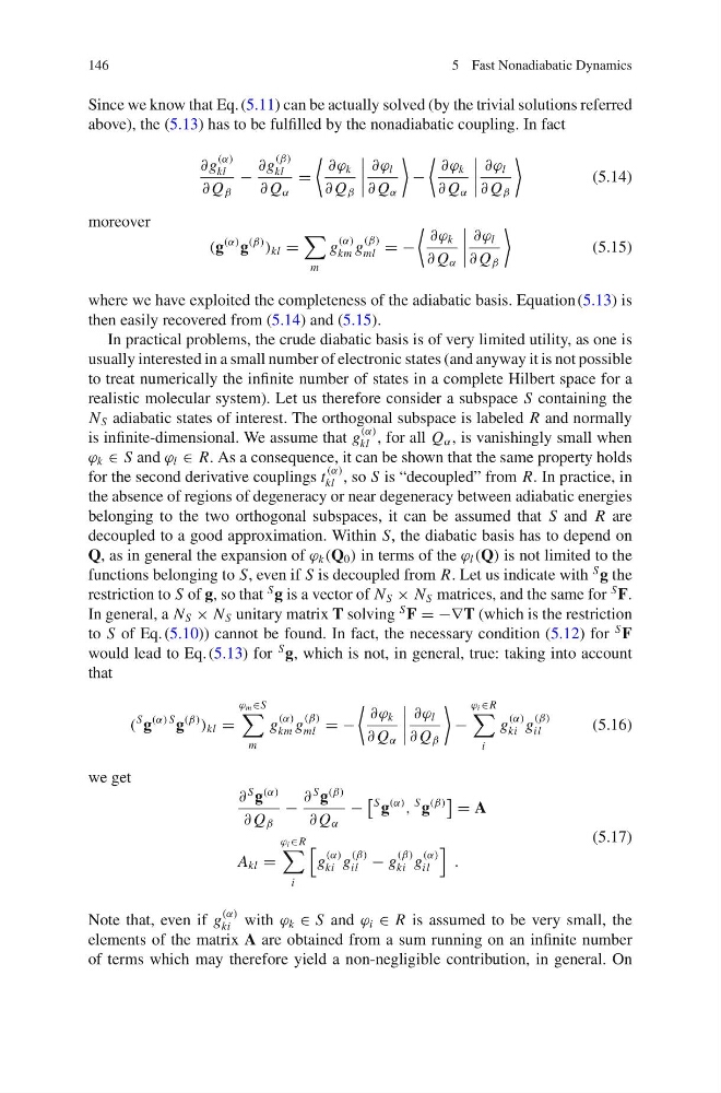
Since we know that Eq. (5.11) can be actually solved (by the trivial solutions referred
above), the (5.13) has to be fulfilled by the nonadiabatic coupling. In fact
∂g
(α)
kl
∂ Q β
−
∂g
(β)
kl
∂ Q α
=
∂ϕ k
∂ Q β
∂ϕ l
∂ Q α
−
∂ϕ k
∂ Q α
∂ϕ l
∂ Q β
(5.14)
moreover
(g
(α) g
(β)
) kl =
m
g
(α)
km g
(β)
ml = −
∂ϕ k
∂ Q α
∂ϕ l
∂ Q β
(5.15)
where we have exploited the completeness of the adiabatic basis. Equation (5.13) is
then easily recovered from (5.14) and (5.15).
In practical problems, the crude diabatic basis is of very limited utility, as one is
usually interested in a small number of electronic states (and anyway it is not possible
to treat numerically the infinite number of states in a complete Hilbert space for a
realistic molecular system). Let us therefore consider a subspace S containing the
N S adiabatic states of interest. The orthogonal subspace is labeled R and normally
is infinite-dimensional. We assume that g
(α)
kl , for all Q α , is vanishingly small when
ϕ k ∈ S and ϕ l ∈ R. As a consequence, it can be shown that the same property holds
for the second derivative couplings t
(α)
kl , so S is “decoupled” from R. In practice, in
the absence of regions of degeneracy or near degeneracy between adiabatic energies
belonging to the two orthogonal subspaces, it can be assumed that S and R are
decoupled to a good approximation. Within S, the diabatic basis has to depend on
Q, as in general the expansion of ϕ k (Q 0 ) in terms of the ϕ l (Q) is not limited to the
functions belonging to S, even if S is decoupled from R. Let us indicate with
S g the
restriction to S of g, so that
S g is a vector of N S × N S matrices, and the same for
S F.
In general, a N S × N S unitary matrix T solving
S F = −∇T (which is the restriction
to S of Eq. (5.10)) cannot be found. In fact, the necessary condition (5.12) for
S F
would lead to Eq. (5.13) for
S g, which is not, in general, true: taking into account
that
(
S g
(α) S g
(β)
) kl =
ϕ m ∈S
m
g
(α)
km g
(β)
ml = −
∂ϕ k
∂ Q α
∂ϕ l
∂ Q β
−
ϕ i ∈R
i
g
(α)
ki g
(β)
il
(5.16)
we get
∂
S g
(α)
∂ Q β
−
∂
S g
(β)
∂ Q α
−
S g
(α)
,
S g
(β)
= A
A kl =
ϕ i ∈R
i
g
(α)
ki g
(β)
il − g
(β)
ki g
(α)
il
.
(5.17)
Note that, even if g
(α)
ki with ϕ k ∈ S and ϕ i ∈ R is assumed to be very small, the
elements of the matrix A are obtained from a sum running on an infinite number
of terms which may therefore yield a non-negligible contribution, in general. On
5 Fast Nonadiabatic Dynamics
Since we know that Eq. (5.11) can be actually solved (by the trivial solutions referred
above), the (5.13) has to be fulfilled by the nonadiabatic coupling. In fact
∂g
(α)
kl
∂ Q β
−
∂g
(β)
kl
∂ Q α
=
∂ϕ k
∂ Q β
∂ϕ l
∂ Q α
−
∂ϕ k
∂ Q α
∂ϕ l
∂ Q β
(5.14)
moreover
(g
(α) g
(β)
) kl =
m
g
(α)
km g
(β)
ml = −
∂ϕ k
∂ Q α
∂ϕ l
∂ Q β
(5.15)
where we have exploited the completeness of the adiabatic basis. Equation (5.13) is
then easily recovered from (5.14) and (5.15).
In practical problems, the crude diabatic basis is of very limited utility, as one is
usually interested in a small number of electronic states (and anyway it is not possible
to treat numerically the infinite number of states in a complete Hilbert space for a
realistic molecular system). Let us therefore consider a subspace S containing the
N S adiabatic states of interest. The orthogonal subspace is labeled R and normally
is infinite-dimensional. We assume that g
(α)
kl , for all Q α , is vanishingly small when
ϕ k ∈ S and ϕ l ∈ R. As a consequence, it can be shown that the same property holds
for the second derivative couplings t
(α)
kl , so S is “decoupled” from R. In practice, in
the absence of regions of degeneracy or near degeneracy between adiabatic energies
belonging to the two orthogonal subspaces, it can be assumed that S and R are
decoupled to a good approximation. Within S, the diabatic basis has to depend on
Q, as in general the expansion of ϕ k (Q 0 ) in terms of the ϕ l (Q) is not limited to the
functions belonging to S, even if S is decoupled from R. Let us indicate with
S g the
restriction to S of g, so that
S g is a vector of N S × N S matrices, and the same for
S F.
In general, a N S × N S unitary matrix T solving
S F = −∇T (which is the restriction
to S of Eq. (5.10)) cannot be found. In fact, the necessary condition (5.12) for
S F
would lead to Eq. (5.13) for
S g, which is not, in general, true: taking into account
that
(
S g
(α) S g
(β)
) kl =
ϕ m ∈S
m
g
(α)
km g
(β)
ml = −
∂ϕ k
∂ Q α
∂ϕ l
∂ Q β
−
ϕ i ∈R
i
g
(α)
ki g
(β)
il
(5.16)
we get
∂
S g
(α)
∂ Q β
−
∂
S g
(β)
∂ Q α
−
S g
(α)
,
S g
(β)
= A
A kl =
ϕ i ∈R
i
g
(α)
ki g
(β)
il − g
(β)
ki g
(α)
il
.
(5.17)
Note that, even if g
(α)
ki with ϕ k ∈ S and ϕ i ∈ R is assumed to be very small, the
elements of the matrix A are obtained from a sum running on an infinite number
of terms which may therefore yield a non-negligible contribution, in general. On