

3.4 Time-Dependent Perturbation Theory
89
i( =0)
˜
V i0 (−ω i0 )
2
2
2π
.
(3.42)
For a finite time interval, the same must hold for V
i0 , which is always true if t − t 0
is small enough.
3.5 Excitation by a Continuous Wave
As a first example of application of TDPT we shall consider the perturbation caused
by a continuous electromagnetic wave:
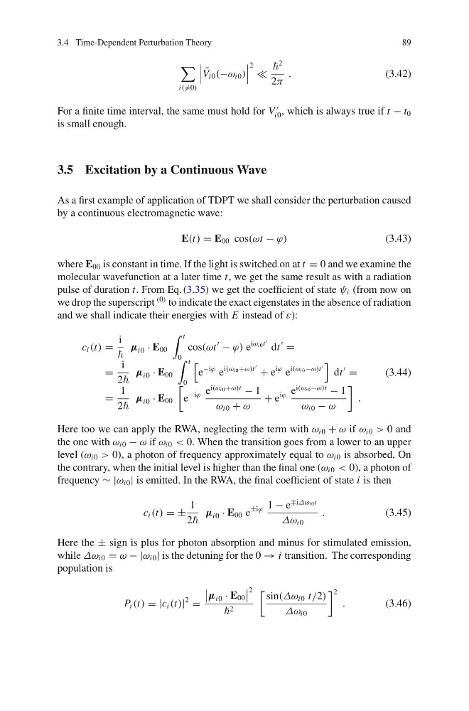
E(t) = E 00 cos(ωt − ϕ)
(3.43)
where E 00 is constant in time. If the light is switched on at t = 0 and we examine the
molecular wavefunction at a later time t, we get the same result as with a radiation
pulse of duration t. From Eq. (3.35) we get the coefficient of state ψ i (from now on
we drop the superscript
(0) to indicate the exact eigenstates in the absence of radiation
and we shall indicate their energies with E instead of ε):
c i (t) =
i
µ i0 · E 00
t
0
cos(ωt
− ϕ) e
iω i0 t
dt
=
=
i
2
µ i0 · E 00
t
0
e
−iϕ e
i(ω i0 +ω)t
+ e
iϕ e
i(ω i0 −ω)t
dt
=
=
1
2
µ i0 · E 00
e
−iϕ e
i(ω i0 +ω)t
− 1
ω i0 + ω
+ e
iϕ e
i(ω i0 −ω)t
− 1
ω i0 − ω
.
(3.44)
Here too we can apply the RWA, neglecting the term with ω i0 + ω if ω i0 > 0 and
the one with ω i0 − ω if ω i0 < 0. When the transition goes from a lower to an upper
level (ω i0 > 0), a photon of frequency approximately equal to ω i0 is absorbed. On
the contrary, when the initial level is higher than the final one (ω i0 < 0), a photon of
frequency ∼ |ω i0 | is emitted. In the RWA, the final coefficient of state i is then
c i (t) = ±
1
2
µ i0 · E 00 e
±iϕ 1 − e
∓iΔω i0 t
Δω i0
.
(3.45)
Here the ± sign is plus for photon absorption and minus for stimulated emission,
while Δω i0 = ω − |ω i0 | is the detuning for the 0 → i transition. The corresponding
population is
P i (t) = |c i (t)|
2
=
µ i0 · E 00
2
2
sin(Δω i0 t/2)
Δω i0
2
.
(3.46)
89
i( =0)
˜
V i0 (−ω i0 )
2
2
2π
.
(3.42)
For a finite time interval, the same must hold for V
i0 , which is always true if t − t 0
is small enough.
3.5 Excitation by a Continuous Wave
As a first example of application of TDPT we shall consider the perturbation caused
by a continuous electromagnetic wave:
E(t) = E 00 cos(ωt − ϕ)
(3.43)
where E 00 is constant in time. If the light is switched on at t = 0 and we examine the
molecular wavefunction at a later time t, we get the same result as with a radiation
pulse of duration t. From Eq. (3.35) we get the coefficient of state ψ i (from now on
we drop the superscript
(0) to indicate the exact eigenstates in the absence of radiation
and we shall indicate their energies with E instead of ε):
c i (t) =
i
µ i0 · E 00
t
0
cos(ωt
− ϕ) e
iω i0 t
dt
=
=
i
2
µ i0 · E 00
t
0
e
−iϕ e
i(ω i0 +ω)t
+ e
iϕ e
i(ω i0 −ω)t
dt
=
=
1
2
µ i0 · E 00
e
−iϕ e
i(ω i0 +ω)t
− 1
ω i0 + ω
+ e
iϕ e
i(ω i0 −ω)t
− 1
ω i0 − ω
.
(3.44)
Here too we can apply the RWA, neglecting the term with ω i0 + ω if ω i0 > 0 and
the one with ω i0 − ω if ω i0 < 0. When the transition goes from a lower to an upper
level (ω i0 > 0), a photon of frequency approximately equal to ω i0 is absorbed. On
the contrary, when the initial level is higher than the final one (ω i0 < 0), a photon of
frequency ∼ |ω i0 | is emitted. In the RWA, the final coefficient of state i is then
c i (t) = ±
1
2
µ i0 · E 00 e
±iϕ 1 − e
∓iΔω i0 t
Δω i0
.
(3.45)
Here the ± sign is plus for photon absorption and minus for stimulated emission,
while Δω i0 = ω − |ω i0 | is the detuning for the 0 → i transition. The corresponding
population is
P i (t) = |c i (t)|
2
=
µ i0 · E 00
2
2
sin(Δω i0 t/2)
Δω i0
2
.
(3.46)