

88
3 Electronic Excitation and Decay
c i (t) = −
i
t
t 0
e
iω i0 t
V i0 (t
) dt
∀ i = 0 .
(3.35)
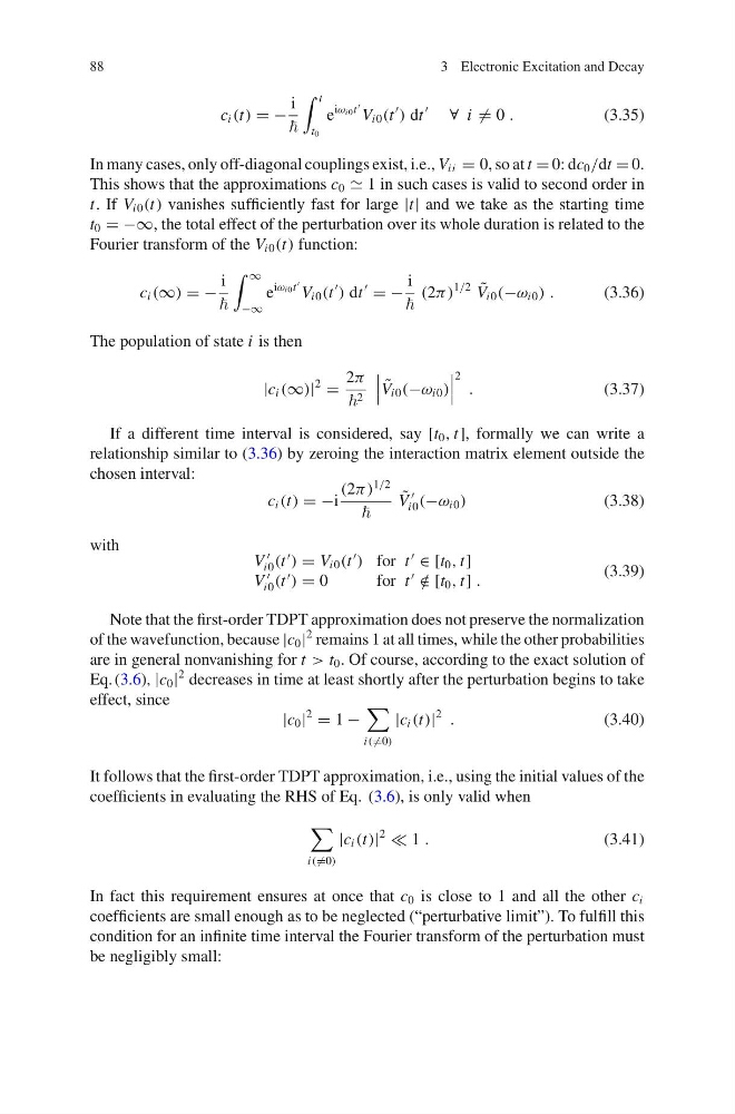
In many cases, only off-diagonal couplings exist, i.e., V ii = 0, so at t = 0: dc 0 /dt = 0.
This shows that the approximations c 0 1 in such cases is valid to second order in
t. If V i0 (t) vanishes sufficiently fast for large |t| and we take as the starting time
t 0 = −∞, the total effect of the perturbation over its whole duration is related to the
Fourier transform of the V i0 (t) function:
c i (∞) = −
i
∞
−∞
e
iω i0 t
V i0 (t
) dt
= −
i
(2π)
1/2 ˜
V i0 (−ω i0 ) .
(3.36)
The population of state i is then
|c i (∞)|
2
=
2π
2
˜
V i0 (−ω i0 )
2 .
(3.37)
If a different time interval is considered, say [t 0 , t], formally we can write a
relationship similar to (3.36) by zeroing the interaction matrix element outside the
chosen interval:
c i (t) = −i
(2π)
1/2
˜
V
i0 (−ω i0 )
(3.38)
with
V
i0 (t
) = V i0 (t
) for t
∈ [t 0 , t]
V
i0 (t
) = 0
for t
/
∈ [t 0 , t] .
(3.39)
Note that the first-order TDPT approximation does not preserve the normalization
of the wavefunction, because |c 0 |
2 remains 1 at all times, while the other probabilities
are in general nonvanishing for t > t 0 . Of course, according to the exact solution of
Eq. (3.6), |c 0 |
2 decreases in time at least shortly after the perturbation begins to take
effect, since
|c 0 |
2
= 1 −
i( =0)
|c i (t)|
2
.
(3.40)
It follows that the first-order TDPT approximation, i.e., using the initial values of the
coefficients in evaluating the RHS of Eq. (3.6), is only valid when
i( =0)
|c i (t)|
2
1 .
(3.41)
In fact this requirement ensures at once that c 0 is close to 1 and all the other c i
coefficients are small enough as to be neglected (“perturbative limit”). To fulfill this
condition for an infinite time interval the Fourier transform of the perturbation must
be negligibly small:
3 Electronic Excitation and Decay
c i (t) = −
i
t
t 0
e
iω i0 t
V i0 (t
) dt
∀ i = 0 .
(3.35)
In many cases, only off-diagonal couplings exist, i.e., V ii = 0, so at t = 0: dc 0 /dt = 0.
This shows that the approximations c 0 1 in such cases is valid to second order in
t. If V i0 (t) vanishes sufficiently fast for large |t| and we take as the starting time
t 0 = −∞, the total effect of the perturbation over its whole duration is related to the
Fourier transform of the V i0 (t) function:
c i (∞) = −
i
∞
−∞
e
iω i0 t
V i0 (t
) dt
= −
i
(2π)
1/2 ˜
V i0 (−ω i0 ) .
(3.36)
The population of state i is then
|c i (∞)|
2
=
2π
2
˜
V i0 (−ω i0 )
2 .
(3.37)
If a different time interval is considered, say [t 0 , t], formally we can write a
relationship similar to (3.36) by zeroing the interaction matrix element outside the
chosen interval:
c i (t) = −i
(2π)
1/2
˜
V
i0 (−ω i0 )
(3.38)
with
V
i0 (t
) = V i0 (t
) for t
∈ [t 0 , t]
V
i0 (t
) = 0
for t
/
∈ [t 0 , t] .
(3.39)
Note that the first-order TDPT approximation does not preserve the normalization
of the wavefunction, because |c 0 |
2 remains 1 at all times, while the other probabilities
are in general nonvanishing for t > t 0 . Of course, according to the exact solution of
Eq. (3.6), |c 0 |
2 decreases in time at least shortly after the perturbation begins to take
effect, since
|c 0 |
2
= 1 −
i( =0)
|c i (t)|
2
.
(3.40)
It follows that the first-order TDPT approximation, i.e., using the initial values of the
coefficients in evaluating the RHS of Eq. (3.6), is only valid when
i( =0)
|c i (t)|
2
1 .
(3.41)
In fact this requirement ensures at once that c 0 is close to 1 and all the other c i
coefficients are small enough as to be neglected (“perturbative limit”). To fulfill this
condition for an infinite time interval the Fourier transform of the perturbation must
be negligibly small: