

2.4 Numerical Integration of the Schrödinger Equation
71
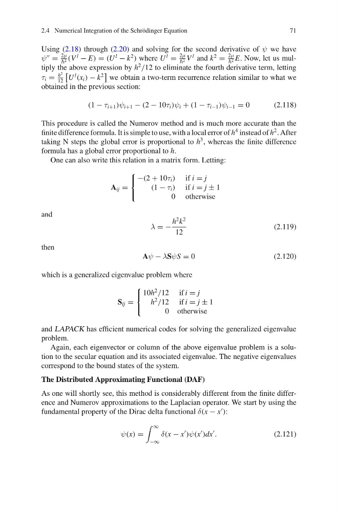
Using (2.18) through (2.20) and solving for the second derivative of ψ we have
ψ
=
2μ
2 (V
l
− E) = (U
l
− k
2
) where U
l
=
2μ
2 V
l and k
2
=
2μ
2 E. Now, let us multiply the above expression by h
2
/12 to eliminate the fourth derivative term, letting
τ i =
h
2
12
U
l
(x i ) − k
2
we obtain a two-term recurrence relation similar to what we
obtained in the previous section:
(1 − τ i+1 )ψ i+1 − (2 − 10τ i )ψ i + (1 − τ i−1 )ψ i−1 = 0
(2.118)
This procedure is called the Numerov method and is much more accurate than the
finite difference formula. It is simple to use, with a local error of h
4 instead of h
2 . After
taking N steps the global error is proportional to h
3 , whereas the finite difference
formula has a global error proportional to h.
One can also write this relation in a matrix form. Letting:
A ij =
⎧
⎨
⎩
−(2 + 10τ i ) if i = j
(1 − τ i ) if i = j ± 1
0 otherwise
and
λ = −
h
2 k
2
12
(2.119)
then
Aψ − λSψS = 0
(2.120)
which is a generalized eigenvalue problem where
S ij =
⎧
⎨
⎩
10h
2
/12 if i = j
h
2
/12 if i = j ± 1
0 otherwise
and LAPACK has efficient numerical codes for solving the generalized eigenvalue
problem.
Again, each eigenvector or column of the above eigenvalue problem is a solution to the secular equation and its associated eigenvalue. The negative eigenvalues
correspond to the bound states of the system.
The Distributed Approximating Functional (DAF)
As one will shortly see, this method is considerably different from the finite difference and Numerov approximations to the Laplacian operator. We start by using the
fundamental property of the Dirac delta functional δ(x − x
):
ψ(x) =
∞
−∞
δ(x − x
)ψ(x
)dx
.
(2.121)
71
Using (2.18) through (2.20) and solving for the second derivative of ψ we have
ψ
=
2μ
2 (V
l
− E) = (U
l
− k
2
) where U
l
=
2μ
2 V
l and k
2
=
2μ
2 E. Now, let us multiply the above expression by h
2
/12 to eliminate the fourth derivative term, letting
τ i =
h
2
12
U
l
(x i ) − k
2
we obtain a two-term recurrence relation similar to what we
obtained in the previous section:
(1 − τ i+1 )ψ i+1 − (2 − 10τ i )ψ i + (1 − τ i−1 )ψ i−1 = 0
(2.118)
This procedure is called the Numerov method and is much more accurate than the
finite difference formula. It is simple to use, with a local error of h
4 instead of h
2 . After
taking N steps the global error is proportional to h
3 , whereas the finite difference
formula has a global error proportional to h.
One can also write this relation in a matrix form. Letting:
A ij =
⎧
⎨
⎩
−(2 + 10τ i ) if i = j
(1 − τ i ) if i = j ± 1
0 otherwise
and
λ = −
h
2 k
2
12
(2.119)
then
Aψ − λSψS = 0
(2.120)
which is a generalized eigenvalue problem where
S ij =
⎧
⎨
⎩
10h
2
/12 if i = j
h
2
/12 if i = j ± 1
0 otherwise
and LAPACK has efficient numerical codes for solving the generalized eigenvalue
problem.
Again, each eigenvector or column of the above eigenvalue problem is a solution to the secular equation and its associated eigenvalue. The negative eigenvalues
correspond to the bound states of the system.
The Distributed Approximating Functional (DAF)
As one will shortly see, this method is considerably different from the finite difference and Numerov approximations to the Laplacian operator. We start by using the
fundamental property of the Dirac delta functional δ(x − x
):
ψ(x) =
∞
−∞
δ(x − x
)ψ(x
)dx
.
(2.121)