

70
2 The Quantum Approach to the Two-Body Problem
• The states with energy less than the asymptotic limits of the potential are bound
states. These states monotonically approach zero in the classically forbidden
regions.
• The states with energy greater than the asymptotic limits of the potential are
continuum states. These states always oscillate in the classically allowed regions
and are characterized by a phase shift.
• The overlap between any two states with different energies and the same effective
potential are orthogonal to each other:
– All bound states are orthonormal to each other
ψ l,E m |ψ l ,E m
= δ m,n δ l,l
– All continuum states are orthogonal to each other
ψ l,E |ψ l,E
= 0 provided that E = E
– All bound and continuum states are orthogonal to each other
ψ l,E n |ψ l ,E
= 0
• It is useful to normalize all bound states to 1
• Continuum states cannot be normalized to 1 but can be normalized in many different ways such as energy normalization
ψ l,E |ψ l,E
= δ(E, E
)
Numerov
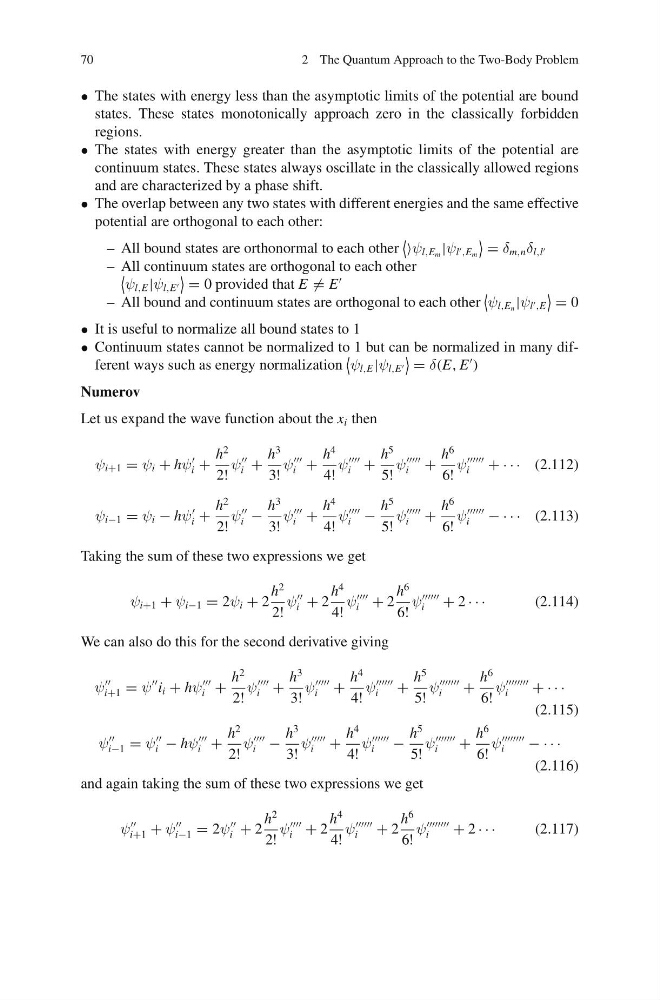
Let us expand the wave function about the x i then
ψ i+1 = ψ i + hψ
i +
h
2
2!
ψ
i +
h
3
3!
ψ
i +
h
4
4!
ψ
i +
h
5
5!
ψ
i
+
h
6
6!
ψ
i
+ · · · (2.112)
ψ i−1 = ψ i − hψ
i +
h
2
2!
ψ
i −
h
3
3!
ψ
i +
h
4
4!
ψ
i −
h
5
5!
ψ
i
+
h
6
6!
ψ
i
− · · · (2.113)
Taking the sum of these two expressions we get
ψ i+1 + ψ i−1 = 2ψ i + 2
h
2
2!
ψ
i + 2
h
4
4!
ψ
i + 2
h
6
6!
ψ
i
+ 2 · · ·
(2.114)
We can also do this for the second derivative giving
ψ
i+1 = ψ
i i + hψ
i +
h
2
2!
ψ
i +
h
3
3!
ψ
i
+
h
4
4!
ψ
i
+
h
5
5!
ψ
i
+
h
6
6!
ψ
i
+ · · ·
(2.115)
ψ
i−1 = ψ
i − hψ
i +
h
2
2!
ψ
i −
h
3
3!
ψ
i
+
h
4
4!
ψ
i
−
h
5
5!
ψ
i
+
h
6
6!
ψ
i
− · · ·
(2.116)
and again taking the sum of these two expressions we get
ψ
i+1 + ψ
i−1 = 2ψ
i + 2
h
2
2!
ψ
i + 2
h
4
4!
ψ
i
+ 2
h
6
6!
ψ
i
+ 2 · · ·
(2.117)
2 The Quantum Approach to the Two-Body Problem
• The states with energy less than the asymptotic limits of the potential are bound
states. These states monotonically approach zero in the classically forbidden
regions.
• The states with energy greater than the asymptotic limits of the potential are
continuum states. These states always oscillate in the classically allowed regions
and are characterized by a phase shift.
• The overlap between any two states with different energies and the same effective
potential are orthogonal to each other:
– All bound states are orthonormal to each other
ψ l,E m |ψ l ,E m
= δ m,n δ l,l
– All continuum states are orthogonal to each other
ψ l,E |ψ l,E
= 0 provided that E = E
– All bound and continuum states are orthogonal to each other
ψ l,E n |ψ l ,E
= 0
• It is useful to normalize all bound states to 1
• Continuum states cannot be normalized to 1 but can be normalized in many different ways such as energy normalization
ψ l,E |ψ l,E
= δ(E, E
)
Numerov
Let us expand the wave function about the x i then
ψ i+1 = ψ i + hψ
i +
h
2
2!
ψ
i +
h
3
3!
ψ
i +
h
4
4!
ψ
i +
h
5
5!
ψ
i
+
h
6
6!
ψ
i
+ · · · (2.112)
ψ i−1 = ψ i − hψ
i +
h
2
2!
ψ
i −
h
3
3!
ψ
i +
h
4
4!
ψ
i −
h
5
5!
ψ
i
+
h
6
6!
ψ
i
− · · · (2.113)
Taking the sum of these two expressions we get
ψ i+1 + ψ i−1 = 2ψ i + 2
h
2
2!
ψ
i + 2
h
4
4!
ψ
i + 2
h
6
6!
ψ
i
+ 2 · · ·
(2.114)
We can also do this for the second derivative giving
ψ
i+1 = ψ
i i + hψ
i +
h
2
2!
ψ
i +
h
3
3!
ψ
i
+
h
4
4!
ψ
i
+
h
5
5!
ψ
i
+
h
6
6!
ψ
i
+ · · ·
(2.115)
ψ
i−1 = ψ
i − hψ
i +
h
2
2!
ψ
i −
h
3
3!
ψ
i
+
h
4
4!
ψ
i
−
h
5
5!
ψ
i
+
h
6
6!
ψ
i
− · · ·
(2.116)
and again taking the sum of these two expressions we get
ψ
i+1 + ψ
i−1 = 2ψ
i + 2
h
2
2!
ψ
i + 2
h
4
4!
ψ
i
+ 2
h
6
6!
ψ
i
+ 2 · · ·
(2.117)