

2.4 Numerical Integration of the Schrödinger Equation
69
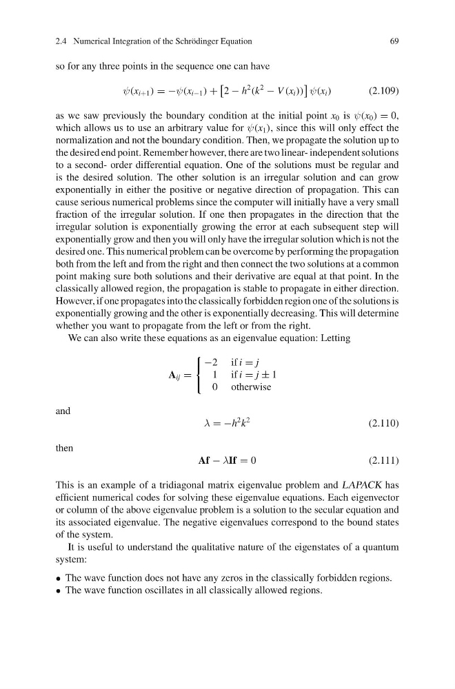
so for any three points in the sequence one can have
ψ(x i+1 ) = −ψ(x i−1 ) +
2 − h
2
(k
2
− V (x i ))
ψ(x i )
(2.109)
as we saw previously the boundary condition at the initial point x 0 is ψ(x 0 ) = 0,
which allows us to use an arbitrary value for ψ(x 1 ), since this will only effect the
normalization and not the boundary condition. Then, we propagate the solution up to
the desired end point. Remember however, there are two linear- independent solutions
to a second- order differential equation. One of the solutions must be regular and
is the desired solution. The other solution is an irregular solution and can grow
exponentially in either the positive or negative direction of propagation. This can
cause serious numerical problems since the computer will initially have a very small
fraction of the irregular solution. If one then propagates in the direction that the
irregular solution is exponentially growing the error at each subsequent step will
exponentially grow and then you will only have the irregular solution which is not the
desired one. This numerical problem can be overcome by performing the propagation
both from the left and from the right and then connect the two solutions at a common
point making sure both solutions and their derivative are equal at that point. In the
classically allowed region, the propagation is stable to propagate in either direction.
However, if one propagates into the classically forbidden region one of the solutions is
exponentially growing and the other is exponentially decreasing. This will determine
whether you want to propagate from the left or from the right.
We can also write these equations as an eigenvalue equation: Letting
A ij =
⎧
⎨
⎩
−2 ifi = j
1 ifi = j ± 1
0 otherwise
and
λ = −h
2 k
2
(2.110)
then
Af − λIf = 0
(2.111)
This is an example of a tridiagonal matrix eigenvalue problem and LAPACK has
efficient numerical codes for solving these eigenvalue equations. Each eigenvector
or column of the above eigenvalue problem is a solution to the secular equation and
its associated eigenvalue. The negative eigenvalues correspond to the bound states
of the system.
It is useful to understand the qualitative nature of the eigenstates of a quantum
system:
• The wave function does not have any zeros in the classically forbidden regions.
• The wave function oscillates in all classically allowed regions.
69
so for any three points in the sequence one can have
ψ(x i+1 ) = −ψ(x i−1 ) +
2 − h
2
(k
2
− V (x i ))
ψ(x i )
(2.109)
as we saw previously the boundary condition at the initial point x 0 is ψ(x 0 ) = 0,
which allows us to use an arbitrary value for ψ(x 1 ), since this will only effect the
normalization and not the boundary condition. Then, we propagate the solution up to
the desired end point. Remember however, there are two linear- independent solutions
to a second- order differential equation. One of the solutions must be regular and
is the desired solution. The other solution is an irregular solution and can grow
exponentially in either the positive or negative direction of propagation. This can
cause serious numerical problems since the computer will initially have a very small
fraction of the irregular solution. If one then propagates in the direction that the
irregular solution is exponentially growing the error at each subsequent step will
exponentially grow and then you will only have the irregular solution which is not the
desired one. This numerical problem can be overcome by performing the propagation
both from the left and from the right and then connect the two solutions at a common
point making sure both solutions and their derivative are equal at that point. In the
classically allowed region, the propagation is stable to propagate in either direction.
However, if one propagates into the classically forbidden region one of the solutions is
exponentially growing and the other is exponentially decreasing. This will determine
whether you want to propagate from the left or from the right.
We can also write these equations as an eigenvalue equation: Letting
A ij =
⎧
⎨
⎩
−2 ifi = j
1 ifi = j ± 1
0 otherwise
and
λ = −h
2 k
2
(2.110)
then
Af − λIf = 0
(2.111)
This is an example of a tridiagonal matrix eigenvalue problem and LAPACK has
efficient numerical codes for solving these eigenvalue equations. Each eigenvector
or column of the above eigenvalue problem is a solution to the secular equation and
its associated eigenvalue. The negative eigenvalues correspond to the bound states
of the system.
It is useful to understand the qualitative nature of the eigenstates of a quantum
system:
• The wave function does not have any zeros in the classically forbidden regions.
• The wave function oscillates in all classically allowed regions.