

2.2 Quantum Elastic Scattering
55
r
z
θ
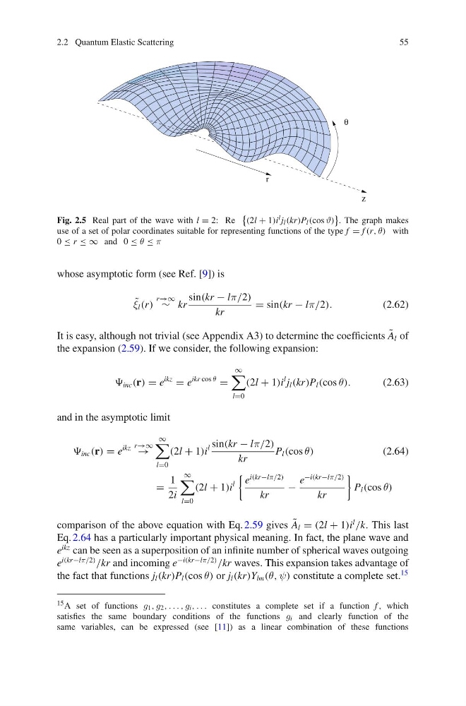
Fig. 2.5 Real part of the wave with l = 2: Re
(2l + 1)i l j l (kr)P l (cos ϑ)
. The graph makes
use of a set of polar coordinates suitable for representing functions of the type f = f (r, θ) with
0 ≤ r ≤ ∞ and 0 ≤ θ ≤ π
whose asymptotic form (see Ref. [9]) is
˜
ξ l (r)
r→∞
∼ kr
sin(kr − lπ/2)
kr
= sin(kr − lπ/2).
(2.62)
It is easy, although not trivial (see Appendix A3) to determine the coefficients ˜
A l of
the expansion (2.59). If we consider, the following expansion:
inc (r) = e
ikz
= e
ikr cos θ
=
∞
l=0
(2l + 1)i
l j l (kr)P l (cos θ).
(2.63)
and in the asymptotic limit
inc (r) = e
ikz r→∞
→
∞
l=0
(2l + 1)i
l sin(kr − lπ/2)
kr
P l (cos θ)
(2.64)
=
1
2i
∞
l=0
(2l + 1)i
l
e
i(kr−lπ/2)
kr
−
e
−i(kr−lπ/2)
kr
P l (cos θ)
comparison of the above equation with Eq. 2.59 gives ˜
A l = (2l + 1)i
l
/k. This last
Eq. 2.64 has a particularly important physical meaning. In fact, the plane wave and
e
ikz can be seen as a superposition of an infinite number of spherical waves outgoing
e
i(kr−lπ/2)
/kr and incoming e
−i(kr−lπ/2)
/kr waves. This expansion takes advantage of
the fact that functions j l (kr)P l (cos θ) or j l (kr)Y lm (θ, ψ) constitute a complete set.
15
15 A set of functions g 1 , g 2 , . . . , g i , . . . constitutes a complete set if a function f , which
satisfies the same boundary conditions of the functions g i and clearly function of the
same variables, can be expressed (see [11]) as a linear combination of these functions
55
r
z
θ
Fig. 2.5 Real part of the wave with l = 2: Re
(2l + 1)i l j l (kr)P l (cos ϑ)
. The graph makes
use of a set of polar coordinates suitable for representing functions of the type f = f (r, θ) with
0 ≤ r ≤ ∞ and 0 ≤ θ ≤ π
whose asymptotic form (see Ref. [9]) is
˜
ξ l (r)
r→∞
∼ kr
sin(kr − lπ/2)
kr
= sin(kr − lπ/2).
(2.62)
It is easy, although not trivial (see Appendix A3) to determine the coefficients ˜
A l of
the expansion (2.59). If we consider, the following expansion:
inc (r) = e
ikz
= e
ikr cos θ
=
∞
l=0
(2l + 1)i
l j l (kr)P l (cos θ).
(2.63)
and in the asymptotic limit
inc (r) = e
ikz r→∞
→
∞
l=0
(2l + 1)i
l sin(kr − lπ/2)
kr
P l (cos θ)
(2.64)
=
1
2i
∞
l=0
(2l + 1)i
l
e
i(kr−lπ/2)
kr
−
e
−i(kr−lπ/2)
kr
P l (cos θ)
comparison of the above equation with Eq. 2.59 gives ˜
A l = (2l + 1)i
l
/k. This last
Eq. 2.64 has a particularly important physical meaning. In fact, the plane wave and
e
ikz can be seen as a superposition of an infinite number of spherical waves outgoing
e
i(kr−lπ/2)
/kr and incoming e
−i(kr−lπ/2)
/kr waves. This expansion takes advantage of
the fact that functions j l (kr)P l (cos θ) or j l (kr)Y lm (θ, ψ) constitute a complete set.
15
15 A set of functions g 1 , g 2 , . . . , g i , . . . constitutes a complete set if a function f , which
satisfies the same boundary conditions of the functions g i and clearly function of the
same variables, can be expressed (see [11]) as a linear combination of these functions