

54
2 The Quantum Approach to the Two-Body Problem
(r)
r→∞
∼ inc (r) + dif (r) = e
ikz
+
1
r
e
ikr f (θ).
(2.56)
The boundary conditions of our problem are the following:
(r) = 0, r → 0
(r) = inc (r) + dif (r) = e
ikz
+
1
r
e
ikr f (θ), r → ∞
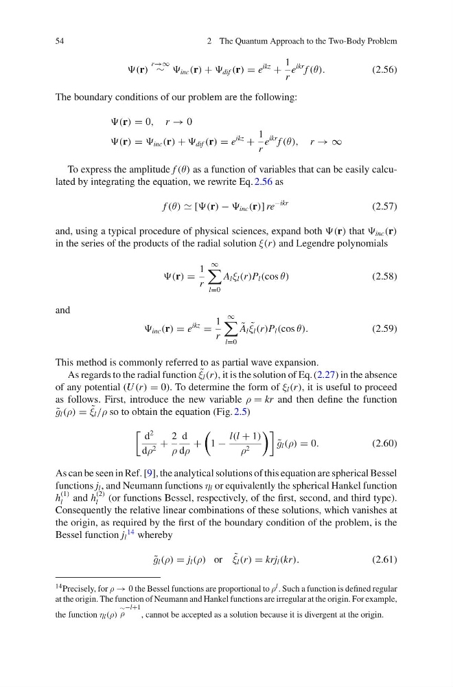
To express the amplitude f (θ) as a function of variables that can be easily calculated by integrating the equation, we rewrite Eq. 2.56 as
f (θ) [(r) − inc (r)] re
−ikr
(2.57)
and, using a typical procedure of physical sciences, expand both (r) that inc (r)
in the series of the products of the radial solution ξ(r) and Legendre polynomials
(r) =
1
r
∞
l=0
A l ξ l (r)P l (cos θ)
(2.58)
and
inc (r) = e
ikz
=
1
r
∞
l=0
˜
A l ˜
ξ l (r)P l (cos θ).
(2.59)
This method is commonly referred to as partial wave expansion.
As regards to the radial function ˜
ξ l (r), it is the solution of Eq. (2.27) in the absence
of any potential (U (r) = 0). To determine the form of ξ l (r), it is useful to proceed
as follows. First, introduce the new variable ρ = kr and then define the function
˜
g l (ρ) = ˜
ξ l /ρ so to obtain the equation (Fig. 2.5)
d
2
dρ 2 +
2
ρ
d
dρ
+
1 −
l(l + 1)
ρ 2
˜
g l (ρ) = 0.
(2.60)
As can be seen in Ref. [9], the analytical solutions of this equation are spherical Bessel
functions j l , and Neumann functions η l or equivalently the spherical Hankel function
h
(1)
l and h
(2)
l (or functions Bessel, respectively, of the first, second, and third type).
Consequently the relative linear combinations of these solutions, which vanishes at
the origin, as required by the first of the boundary condition of the problem, is the
Bessel function j l
14 whereby
˜
g l (ρ) = j l (ρ) or ˜
ξ l (r) = krj l (kr).
(2.61)
14 Precisely, for ρ → 0 the Bessel functions are proportional to ρ l . Such a function is defined regular
at the origin. The function of Neumann and Hankel functions are irregular at the origin. For example,
the function η l (ρ)
∼
ρ
−l+1
, cannot be accepted as a solution because it is divergent at the origin.
2 The Quantum Approach to the Two-Body Problem
(r)
r→∞
∼ inc (r) + dif (r) = e
ikz
+
1
r
e
ikr f (θ).
(2.56)
The boundary conditions of our problem are the following:
(r) = 0, r → 0
(r) = inc (r) + dif (r) = e
ikz
+
1
r
e
ikr f (θ), r → ∞
To express the amplitude f (θ) as a function of variables that can be easily calculated by integrating the equation, we rewrite Eq. 2.56 as
f (θ) [(r) − inc (r)] re
−ikr
(2.57)
and, using a typical procedure of physical sciences, expand both (r) that inc (r)
in the series of the products of the radial solution ξ(r) and Legendre polynomials
(r) =
1
r
∞
l=0
A l ξ l (r)P l (cos θ)
(2.58)
and
inc (r) = e
ikz
=
1
r
∞
l=0
˜
A l ˜
ξ l (r)P l (cos θ).
(2.59)
This method is commonly referred to as partial wave expansion.
As regards to the radial function ˜
ξ l (r), it is the solution of Eq. (2.27) in the absence
of any potential (U (r) = 0). To determine the form of ξ l (r), it is useful to proceed
as follows. First, introduce the new variable ρ = kr and then define the function
˜
g l (ρ) = ˜
ξ l /ρ so to obtain the equation (Fig. 2.5)
d
2
dρ 2 +
2
ρ
d
dρ
+
1 −
l(l + 1)
ρ 2
˜
g l (ρ) = 0.
(2.60)
As can be seen in Ref. [9], the analytical solutions of this equation are spherical Bessel
functions j l , and Neumann functions η l or equivalently the spherical Hankel function
h
(1)
l and h
(2)
l (or functions Bessel, respectively, of the first, second, and third type).
Consequently the relative linear combinations of these solutions, which vanishes at
the origin, as required by the first of the boundary condition of the problem, is the
Bessel function j l
14 whereby
˜
g l (ρ) = j l (ρ) or ˜
ξ l (r) = krj l (kr).
(2.61)
14 Precisely, for ρ → 0 the Bessel functions are proportional to ρ l . Such a function is defined regular
at the origin. The function of Neumann and Hankel functions are irregular at the origin. For example,
the function η l (ρ)
∼
ρ
−l+1
, cannot be accepted as a solution because it is divergent at the origin.