

52
2 The Quantum Approach to the Two-Body Problem
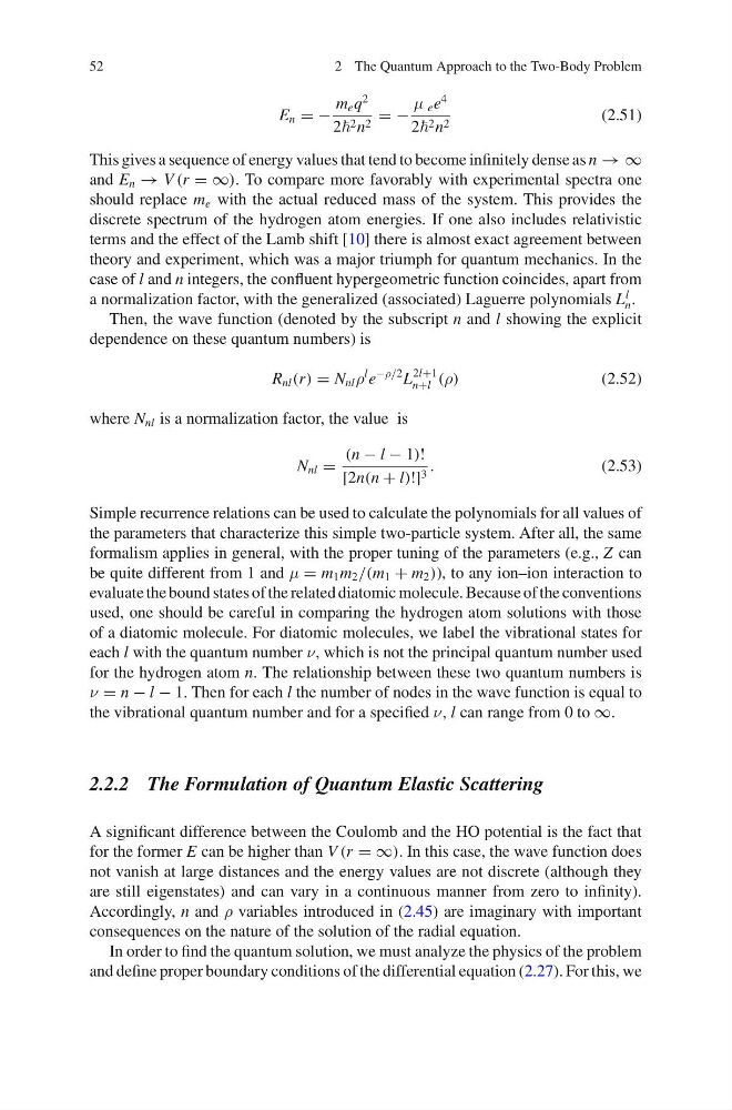
E n = −
m e q
2
2 2 n 2 = −
μ e e
4
2 2 n 2
(2.51)
This gives a sequence of energy values that tend to become infinitely dense as n → ∞
and E n → V (r = ∞). To compare more favorably with experimental spectra one
should replace m e with the actual reduced mass of the system. This provides the
discrete spectrum of the hydrogen atom energies. If one also includes relativistic
terms and the effect of the Lamb shift [10] there is almost exact agreement between
theory and experiment, which was a major triumph for quantum mechanics. In the
case of l and n integers, the confluent hypergeometric function coincides, apart from
a normalization factor, with the generalized (associated) Laguerre polynomials L
l
n .
Then, the wave function (denoted by the subscript n and l showing the explicit
dependence on these quantum numbers) is
R nl (r) = N nl ρ
l e
−ρ/2 L
2l+1
n+l (ρ)
(2.52)
where N nl is a normalization factor, the value is
N nl =
(n − l − 1)!
[2n(n + l)!] 3 .
(2.53)
Simple recurrence relations can be used to calculate the polynomials for all values of
the parameters that characterize this simple two-particle system. After all, the same
formalism applies in general, with the proper tuning of the parameters (e.g., Z can
be quite different from 1 and μ = m 1 m 2 /(m 1 + m 2 )), to any ion–ion interaction to
evaluate the bound states of the related diatomic molecule. Because of the conventions
used, one should be careful in comparing the hydrogen atom solutions with those
of a diatomic molecule. For diatomic molecules, we label the vibrational states for
each l with the quantum number ν, which is not the principal quantum number used
for the hydrogen atom n. The relationship between these two quantum numbers is
ν = n − l − 1. Then for each l the number of nodes in the wave function is equal to
the vibrational quantum number and for a specified ν, l can range from 0 to ∞.
2.2.2 The Formulation of Quantum Elastic Scattering
A significant difference between the Coulomb and the HO potential is the fact that
for the former E can be higher than V (r = ∞). In this case, the wave function does
not vanish at large distances and the energy values are not discrete (although they
are still eigenstates) and can vary in a continuous manner from zero to infinity).
Accordingly, n and ρ variables introduced in (2.45) are imaginary with important
consequences on the nature of the solution of the radial equation.
In order to find the quantum solution, we must analyze the physics of the problem
and define proper boundary conditions of the differential equation (2.27). For this, we
2 The Quantum Approach to the Two-Body Problem
E n = −
m e q
2
2 2 n 2 = −
μ e e
4
2 2 n 2
(2.51)
This gives a sequence of energy values that tend to become infinitely dense as n → ∞
and E n → V (r = ∞). To compare more favorably with experimental spectra one
should replace m e with the actual reduced mass of the system. This provides the
discrete spectrum of the hydrogen atom energies. If one also includes relativistic
terms and the effect of the Lamb shift [10] there is almost exact agreement between
theory and experiment, which was a major triumph for quantum mechanics. In the
case of l and n integers, the confluent hypergeometric function coincides, apart from
a normalization factor, with the generalized (associated) Laguerre polynomials L
l
n .
Then, the wave function (denoted by the subscript n and l showing the explicit
dependence on these quantum numbers) is
R nl (r) = N nl ρ
l e
−ρ/2 L
2l+1
n+l (ρ)
(2.52)
where N nl is a normalization factor, the value is
N nl =
(n − l − 1)!
[2n(n + l)!] 3 .
(2.53)
Simple recurrence relations can be used to calculate the polynomials for all values of
the parameters that characterize this simple two-particle system. After all, the same
formalism applies in general, with the proper tuning of the parameters (e.g., Z can
be quite different from 1 and μ = m 1 m 2 /(m 1 + m 2 )), to any ion–ion interaction to
evaluate the bound states of the related diatomic molecule. Because of the conventions
used, one should be careful in comparing the hydrogen atom solutions with those
of a diatomic molecule. For diatomic molecules, we label the vibrational states for
each l with the quantum number ν, which is not the principal quantum number used
for the hydrogen atom n. The relationship between these two quantum numbers is
ν = n − l − 1. Then for each l the number of nodes in the wave function is equal to
the vibrational quantum number and for a specified ν, l can range from 0 to ∞.
2.2.2 The Formulation of Quantum Elastic Scattering
A significant difference between the Coulomb and the HO potential is the fact that
for the former E can be higher than V (r = ∞). In this case, the wave function does
not vanish at large distances and the energy values are not discrete (although they
are still eigenstates) and can vary in a continuous manner from zero to infinity).
Accordingly, n and ρ variables introduced in (2.45) are imaginary with important
consequences on the nature of the solution of the radial equation.
In order to find the quantum solution, we must analyze the physics of the problem
and define proper boundary conditions of the differential equation (2.27). For this, we