

1.4 Popular Scattering Model Potentials
35
In the case of the LJ potential, the integral of Eq. 1.44 does not admit analytical
solution. Accordingly, the calculation of θ is only possible using digital techniques.
Anyway, it is instructive to compare the shape of this potential by plotting its value
as a function of the impact parameter so as to highlight the effect of the angular
momentum term on the effective potential V
l
(r ) (see Eq. 1.41). The Hamiltonian
of the system (see Eq. 1.33) can in fact be conveniently rewritten by expressing the
angular velocity in terms of the two-body total angular momentum L (Eq. (1.40)
from which ˙
θ = l/μr
2 ) leading to the following expression:
H =
1
2
μ˙ r
2
+
l
2
2μr 2 + V (r ) =
1
2
μ˙ r
2
+ V
l
(r ).
(1.74)
The proper way to scale the Lennard–Jones potential is to divide the radial distances
by the parameter σ (r
∗
= r/σ and b
∗
= b/σ) and the energies by the parameter
(V
∗
= V / and E
∗
= E/). The scaled quantities are marked with an asterisk.
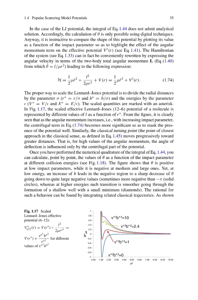
In Fig. 1.17, the scaled effective Lennard–Jones (12–6) potential of a molecule is
represented by different values of l as a function of r
∗ . From the figure, it is clearly
seen that as the angular momentum increases, i.e., with increasing impact parameter,
the centrifugal term in Eq. (1.74) becomes more significant so as to mask the presence of the potential well. Similarly, the classical turning point (the point of closest
approach in the classical sense, as defined in Eq. 1.45) moves progressively toward
greater distances. That is, for high values of the angular momentum, the angle of
deflection is influenced only by the centrifugal part of the potential.
Once you have performed the numerical quadrature of the integral of Eq. 1.44, you
can calculate, point by point, the values of θ as a function of the impact parameter
at different collision energies (see Fig. 1.18). The figure shows that θ is positive
at low impact parameters, while it is negative at medium and large ones. Yet, at
low energy, an increase of b leads in the negative region to a sharp decrease of θ
going down to quite large negative values (sometimes more negative than −π (solid
circles), whereas at higher energies such transition is smoother going through the
formation of a shallow well with a small minimum (diamonds). The rational for
such a behavior can be found by integrating related classical trajectories. As shown
Fig. 1.17 Scaled
Lennard–Jones effective
potential (6–12):
V
∗
ef f (r ) = V (r
∗ ) +
l 2
2μr ∗ 2 =
V (r
∗ ) +
v ∗ 2 b ∗ 2
r ∗ 2 for different
values of v ∗ 2 b ∗ 2
-1
-0.8
-0.6
-0.4
-0.2
0
0.2
0.4
0.6
0.8
1
0.00
1.00
2.00
3.00
4.00
5.00
6.00
7.00
8.00
9.00 10.00
V*
eff
r*
v* 2 b* 2 =0
v* 2 b* 2 =10
v* 2 b* 2 =2.4
v* 2 b* 2 =1
35
In the case of the LJ potential, the integral of Eq. 1.44 does not admit analytical
solution. Accordingly, the calculation of θ is only possible using digital techniques.
Anyway, it is instructive to compare the shape of this potential by plotting its value
as a function of the impact parameter so as to highlight the effect of the angular
momentum term on the effective potential V
l
(r ) (see Eq. 1.41). The Hamiltonian
of the system (see Eq. 1.33) can in fact be conveniently rewritten by expressing the
angular velocity in terms of the two-body total angular momentum L (Eq. (1.40)
from which ˙
θ = l/μr
2 ) leading to the following expression:
H =
1
2
μ˙ r
2
+
l
2
2μr 2 + V (r ) =
1
2
μ˙ r
2
+ V
l
(r ).
(1.74)
The proper way to scale the Lennard–Jones potential is to divide the radial distances
by the parameter σ (r
∗
= r/σ and b
∗
= b/σ) and the energies by the parameter
(V
∗
= V / and E
∗
= E/). The scaled quantities are marked with an asterisk.
In Fig. 1.17, the scaled effective Lennard–Jones (12–6) potential of a molecule is
represented by different values of l as a function of r
∗ . From the figure, it is clearly
seen that as the angular momentum increases, i.e., with increasing impact parameter,
the centrifugal term in Eq. (1.74) becomes more significant so as to mask the presence of the potential well. Similarly, the classical turning point (the point of closest
approach in the classical sense, as defined in Eq. 1.45) moves progressively toward
greater distances. That is, for high values of the angular momentum, the angle of
deflection is influenced only by the centrifugal part of the potential.
Once you have performed the numerical quadrature of the integral of Eq. 1.44, you
can calculate, point by point, the values of θ as a function of the impact parameter
at different collision energies (see Fig. 1.18). The figure shows that θ is positive
at low impact parameters, while it is negative at medium and large ones. Yet, at
low energy, an increase of b leads in the negative region to a sharp decrease of θ
going down to quite large negative values (sometimes more negative than −π (solid
circles), whereas at higher energies such transition is smoother going through the
formation of a shallow well with a small minimum (diamonds). The rational for
such a behavior can be found by integrating related classical trajectories. As shown
Fig. 1.17 Scaled
Lennard–Jones effective
potential (6–12):
V
∗
ef f (r ) = V (r
∗ ) +
l 2
2μr ∗ 2 =
V (r
∗ ) +
v ∗ 2 b ∗ 2
r ∗ 2 for different
values of v ∗ 2 b ∗ 2
-1
-0.8
-0.6
-0.4
-0.2
0
0.2
0.4
0.6
0.8
1
0.00
1.00
2.00
3.00
4.00
5.00
6.00
7.00
8.00
9.00 10.00
V*
eff
r*
v* 2 b* 2 =0
v* 2 b* 2 =10
v* 2 b* 2 =2.4
v* 2 b* 2 =1