

1.4 Popular Scattering Model Potentials
33
0.0
1.0
2.0
3.0
4.0
5.0
6.0
7.0
8.0
9.0 10.0
-5.0
-4.0
-3.0
-2.0
-1.0
0.0
1.0
2.0
3.0
4.0
R e
V(R)/eV
R/A
D=4.621
R e =0.970
D
Morse Potential for OH
0
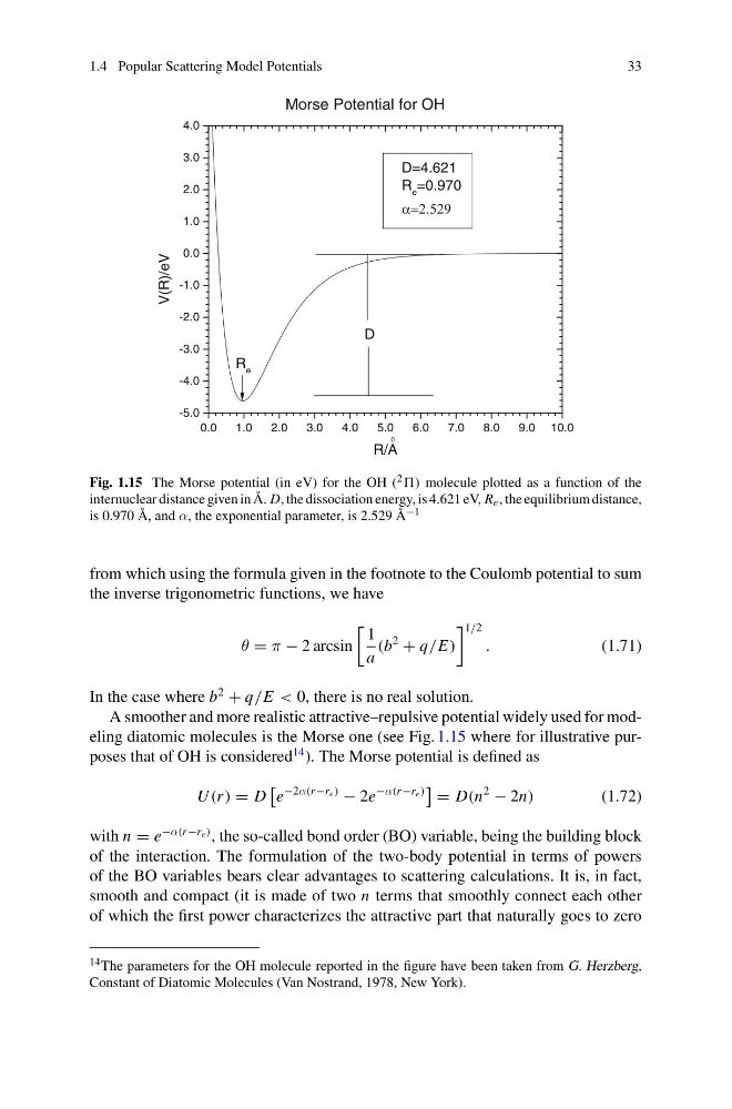
Fig. 1.15 The Morse potential (in eV) for the OH ( 2 ) molecule plotted as a function of the
internuclear distance given in Å. D, the dissociation energy, is 4.621 eV, R e , the equilibrium distance,
is 0.970 Å, and α, the exponential parameter, is 2.529 Å −1
from which using the formula given in the footnote to the Coulomb potential to sum
the inverse trigonometric functions, we have
θ = π − 2 arcsin
1
a
(b
2
+ q/E)
1/2
.
(1.71)
In the case where b
2
+ q/E < 0, there is no real solution.
A smoother and more realistic attractive–repulsive potential widely used for modeling diatomic molecules is the Morse one (see Fig. 1.15 where for illustrative purposes that of OH is considered
14 ). The Morse potential is defined as
U (r ) = D
e
−2α(r −r e )
− 2e
−α(r −r e )
= D(n
2
− 2n)
(1.72)
with n = e
−α(r −r e ) , the so-called bond order (BO) variable, being the building block
of the interaction. The formulation of the two-body potential in terms of powers
of the BO variables bears clear advantages to scattering calculations. It is, in fact,
smooth and compact (it is made of two n terms that smoothly connect each other
of which the first power characterizes the attractive part that naturally goes to zero
14 The parameters for the OH molecule reported in the figure have been taken from G. Herzberg,
Constant of Diatomic Molecules (Van Nostrand, 1978, New York).
33
0.0
1.0
2.0
3.0
4.0
5.0
6.0
7.0
8.0
9.0 10.0
-5.0
-4.0
-3.0
-2.0
-1.0
0.0
1.0
2.0
3.0
4.0
R e
V(R)/eV
R/A
D=4.621
R e =0.970
D
Morse Potential for OH
0
Fig. 1.15 The Morse potential (in eV) for the OH ( 2 ) molecule plotted as a function of the
internuclear distance given in Å. D, the dissociation energy, is 4.621 eV, R e , the equilibrium distance,
is 0.970 Å, and α, the exponential parameter, is 2.529 Å −1
from which using the formula given in the footnote to the Coulomb potential to sum
the inverse trigonometric functions, we have
θ = π − 2 arcsin
1
a
(b
2
+ q/E)
1/2
.
(1.71)
In the case where b
2
+ q/E < 0, there is no real solution.
A smoother and more realistic attractive–repulsive potential widely used for modeling diatomic molecules is the Morse one (see Fig. 1.15 where for illustrative purposes that of OH is considered
14 ). The Morse potential is defined as
U (r ) = D
e
−2α(r −r e )
− 2e
−α(r −r e )
= D(n
2
− 2n)
(1.72)
with n = e
−α(r −r e ) , the so-called bond order (BO) variable, being the building block
of the interaction. The formulation of the two-body potential in terms of powers
of the BO variables bears clear advantages to scattering calculations. It is, in fact,
smooth and compact (it is made of two n terms that smoothly connect each other
of which the first power characterizes the attractive part that naturally goes to zero
14 The parameters for the OH molecule reported in the figure have been taken from G. Herzberg,
Constant of Diatomic Molecules (Van Nostrand, 1978, New York).