

1.4 Popular Scattering Model Potentials
31
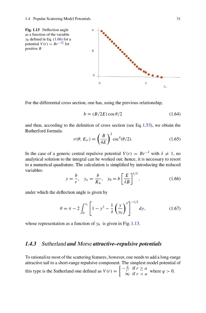
Fig. 1.13 Deflection angle
as a function of the variable
y 0 defined in Eq. (1.66) for a
potential V (r ) = Br −12 for
positive B
0
0
y o
1
For the differential cross section, one has, using the previous relationship,
b = (B/2E) cos θ/2
(1.64)
and then, according to the definition of cross section (see Eq. 1.53), we obtain the
Rutherford formula:
σ(θ, E tr ) =
B
4E
2
csc
4
(θ/2).
(1.65)
In the case of a generic central repulsive potential V (r ) = Br
−δ with δ = 1, no
analytical solution to the integral can be worked out; hence, it is necessary to resort
to a numerical quadrature. The calculation is simplified by introducing the reduced
variables:
y =
b
r
, y a =
b
R A
, y 0 = b
E
δ B
1/δ
,
(1.66)
under which the deflection angle is given by
θ = π − 2
y a
0
1 − y
2
−
1
δ
y
y 0
δ
−1/2
dy,
(1.67)
whose representation as a function of y 0 is given in Fig. 1.13.
1.4.3 Sutherland and Morse attractive–repulsive potentials
To rationalize most of the scattering features, however, one needs to add a long-range
attractive tail to a short-range repulsive component. The simplest model potential of
this type is the Sutherland one defined as V (r ) =
−
q
r γ if r ≥ a
∞ if r < a
where q > 0.
31
Fig. 1.13 Deflection angle
as a function of the variable
y 0 defined in Eq. (1.66) for a
potential V (r ) = Br −12 for
positive B
0
0
y o
1
For the differential cross section, one has, using the previous relationship,
b = (B/2E) cos θ/2
(1.64)
and then, according to the definition of cross section (see Eq. 1.53), we obtain the
Rutherford formula:
σ(θ, E tr ) =
B
4E
2
csc
4
(θ/2).
(1.65)
In the case of a generic central repulsive potential V (r ) = Br
−δ with δ = 1, no
analytical solution to the integral can be worked out; hence, it is necessary to resort
to a numerical quadrature. The calculation is simplified by introducing the reduced
variables:
y =
b
r
, y a =
b
R A
, y 0 = b
E
δ B
1/δ
,
(1.66)
under which the deflection angle is given by
θ = π − 2
y a
0
1 − y
2
−
1
δ
y
y 0
δ
−1/2
dy,
(1.67)
whose representation as a function of y 0 is given in Fig. 1.13.
1.4.3 Sutherland and Morse attractive–repulsive potentials
To rationalize most of the scattering features, however, one needs to add a long-range
attractive tail to a short-range repulsive component. The simplest model potential of
this type is the Sutherland one defined as V (r ) =
−
q
r γ if r ≥ a
∞ if r < a
where q > 0.