

158
5 Complex Reactive Applications: A Forward Look to Open Science
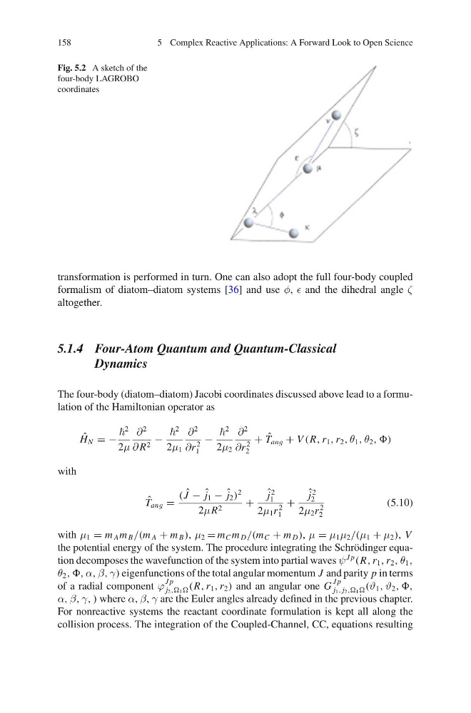
Fig. 5.2 A sketch of the
four-body LAGROBO
coordinates
transformation is performed in turn. One can also adopt the full four-body coupled
formalism of diatom–diatom systems [36] and use φ, and the dihedral angle ζ
altogether.
5.1.4 Four-Atom Quantum and Quantum-Classical
Dynamics
The four-body (diatom–diatom) Jacobi coordinates discussed above lead to a formulation of the Hamiltonian operator as
ˆ
H N = −
2
2μ
∂
2
∂ R 2 −
2
2μ 1
∂
2
∂r
2
1
−
2
2μ 2
∂
2
∂r
2
2
+ ˆ
T ang + V (R, r 1 , r 2 , θ 1 , θ 2 , ,)
with
ˆ
T ang =
( ˆ
J − ˆ
j 1 − ˆ
j 2 )
2
2μR 2
+
ˆ
j
2
1
2μ 1 r
2
1
+
ˆ
j
2
2
2μ 2 r
2
2
(5.10)
with μ 1 = m A m B /(m A + m B ), μ 2 = m C m D /(m C + m D ), μ = μ 1 μ 2 /(μ 1 + μ 2 ), V
the potential energy of the system. The procedure integrating the Schrödinger equation decomposes the wavefunction of the system into partial waves ψ
J p
(R, r 1 , r 2 , θ 1 ,
θ 2 , ,, α, β, γ) eigenfunctions of the total angular momentum J and parity p in terms
of a radial component ϕ
J p
j 2 ,, 1 (R, r 1 , r 2 ) and an angular one G
J p
j 1 , j 2 ,, 1 (ϑ 1 , ϑ 2 , ,,
α, β, γ, ) where α, β, γ are the Euler angles already defined in the previous chapter.
For nonreactive systems the reactant coordinate formulation is kept all along the
collision process. The integration of the Coupled-Channel, CC, equations resulting
5 Complex Reactive Applications: A Forward Look to Open Science
Fig. 5.2 A sketch of the
four-body LAGROBO
coordinates
transformation is performed in turn. One can also adopt the full four-body coupled
formalism of diatom–diatom systems [36] and use φ, and the dihedral angle ζ
altogether.
5.1.4 Four-Atom Quantum and Quantum-Classical
Dynamics
The four-body (diatom–diatom) Jacobi coordinates discussed above lead to a formulation of the Hamiltonian operator as
ˆ
H N = −
2
2μ
∂
2
∂ R 2 −
2
2μ 1
∂
2
∂r
2
1
−
2
2μ 2
∂
2
∂r
2
2
+ ˆ
T ang + V (R, r 1 , r 2 , θ 1 , θ 2 , ,)
with
ˆ
T ang =
( ˆ
J − ˆ
j 1 − ˆ
j 2 )
2
2μR 2
+
ˆ
j
2
1
2μ 1 r
2
1
+
ˆ
j
2
2
2μ 2 r
2
2
(5.10)
with μ 1 = m A m B /(m A + m B ), μ 2 = m C m D /(m C + m D ), μ = μ 1 μ 2 /(μ 1 + μ 2 ), V
the potential energy of the system. The procedure integrating the Schrödinger equation decomposes the wavefunction of the system into partial waves ψ
J p
(R, r 1 , r 2 , θ 1 ,
θ 2 , ,, α, β, γ) eigenfunctions of the total angular momentum J and parity p in terms
of a radial component ϕ
J p
j 2 ,, 1 (R, r 1 , r 2 ) and an angular one G
J p
j 1 , j 2 ,, 1 (ϑ 1 , ϑ 2 , ,,
α, β, γ, ) where α, β, γ are the Euler angles already defined in the previous chapter.
For nonreactive systems the reactant coordinate formulation is kept all along the
collision process. The integration of the Coupled-Channel, CC, equations resulting