

1.1 From Kinetics to Bimolecular Collisions
3
The variation of the intervening species corresponding to that of Eq. 1.1 reads now
v(t) = −
d[A]
αdt
= k[A]
m
[B]
n
,
(1.5)
where m + n is the order of the process with m and n being not necessarily integers.
In the particular case of m=0, 1, and 2, the rate coefficient takes, respectively, the
following analytical forms:
k 0 (T ) =
[A] o − [A]
α(t − t o )
for m = 0,
(1.6)
where [A] o is the concentration of A at the initial time t o and [A] is its concentration
at time t,
k 1 (T ) =
ln[A] o − ln[A]
α(t − t o )
for m = 1
(1.7)
and
k 2 (T ) =
1/[A] o − 1/[A]
α(t − t o )
for m = 2
(1.8)
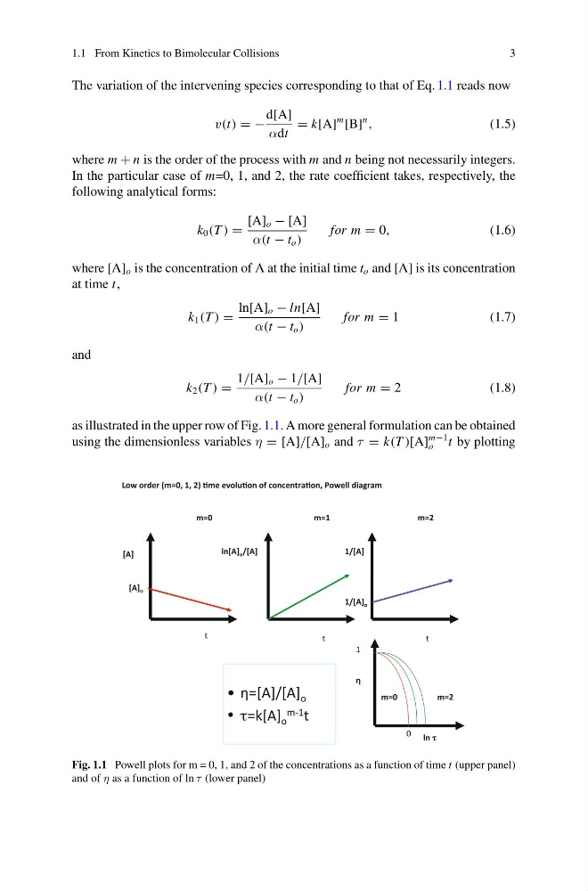
as illustrated in the upper row of Fig. 1.1. A more general formulation can be obtained
using the dimensionless variables η = [A]/[A] o and τ = k(T )[A]
m−1
o
t by plotting
Fig. 1.1 Powell plots for m = 0, 1, and 2 of the concentrations as a function of time t (upper panel)
and of η as a function of ln τ (lower panel)
3
The variation of the intervening species corresponding to that of Eq. 1.1 reads now
v(t) = −
d[A]
αdt
= k[A]
m
[B]
n
,
(1.5)
where m + n is the order of the process with m and n being not necessarily integers.
In the particular case of m=0, 1, and 2, the rate coefficient takes, respectively, the
following analytical forms:
k 0 (T ) =
[A] o − [A]
α(t − t o )
for m = 0,
(1.6)
where [A] o is the concentration of A at the initial time t o and [A] is its concentration
at time t,
k 1 (T ) =
ln[A] o − ln[A]
α(t − t o )
for m = 1
(1.7)
and
k 2 (T ) =
1/[A] o − 1/[A]
α(t − t o )
for m = 2
(1.8)
as illustrated in the upper row of Fig. 1.1. A more general formulation can be obtained
using the dimensionless variables η = [A]/[A] o and τ = k(T )[A]
m−1
o
t by plotting
Fig. 1.1 Powell plots for m = 0, 1, and 2 of the concentrations as a function of time t (upper panel)
and of η as a function of ln τ (lower panel)