

4.2 Three-Atom Systems
123
0
1 0
2 0
3 0
4 0
5 0
6 0
0.00
0.02
0.04
0.06
0.08
0.10
0.12
0.14
0.16
0.18
0.20
0.22
V/eV
Degrees
n=1
n=3
n=5
n=7
n=9
n=11
Odd Vibrational States
0
1 0
2 0
3 0
4 0
5 0
6 0
0.00
0.02
0.04
0.06
0.08
0.10
0.12
0.14
0.16
0.18
0.20
0.22
V/eV
Degrees
Even Vibrational States
n=0
n=2
n=4
n=6
n=8
n=10
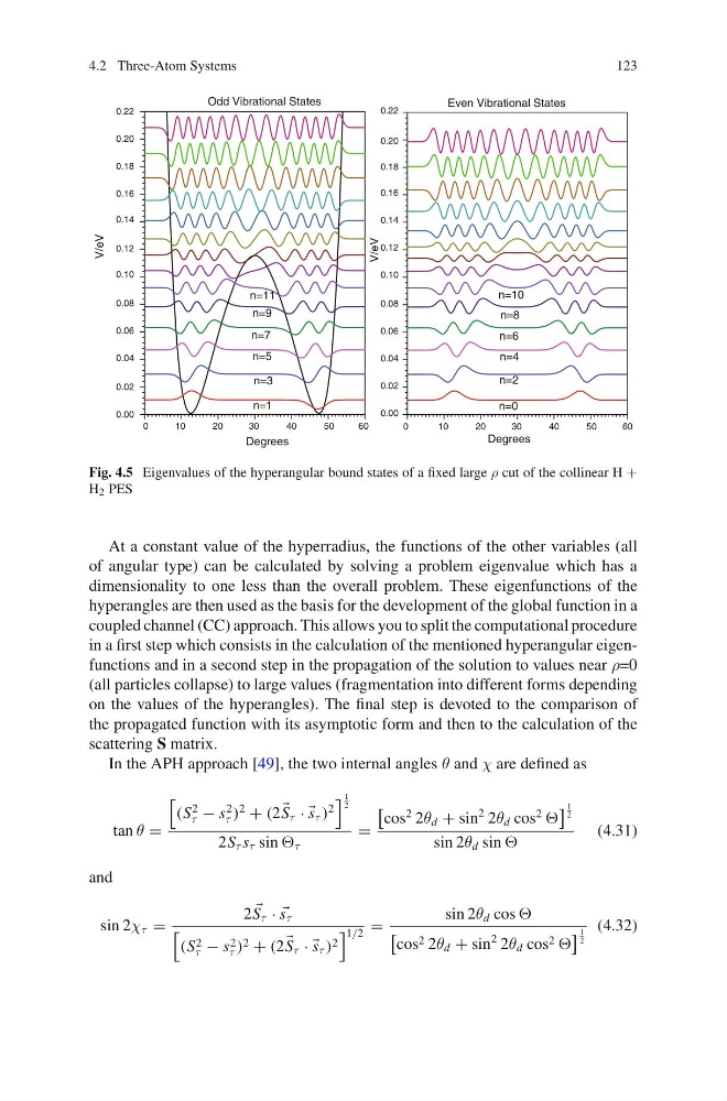
Fig. 4.5 Eigenvalues of the hyperangular bound states of a fixed large ρ cut of the collinear H +
H 2 PES
At a constant value of the hyperradius, the functions of the other variables (all
of angular type) can be calculated by solving a problem eigenvalue which has a
dimensionality to one less than the overall problem. These eigenfunctions of the
hyperangles are then used as the basis for the development of the global function in a
coupled channel (CC) approach. This allows you to split the computational procedure
in a first step which consists in the calculation of the mentioned hyperangular eigenfunctions and in a second step in the propagation of the solution to values near ρ=0
(all particles collapse) to large values (fragmentation into different forms depending
on the values of the hyperangles). The final step is devoted to the comparison of
the propagated function with its asymptotic form and then to the calculation of the
scattering S matrix.
In the APH approach [49], the two internal angles θ and χ are defined as
tan θ =
(S
2
τ − s
2
τ )
2
+ (2
S τ · ·
s τ )
2
1
2
2S τ s τ sin τ
=
cos
2 2θ d + sin
2 2θ d cos
2
1
2
sin 2θ d sin
(4.31)
and
sin 2χ τ =
2
S τ · ·
s τ
(S 2
τ − s 2
τ ) 2 + (2
S τ · ·
s τ ) 2
1/2 =
sin 2θ d cos
cos 2 2θ d + sin
2 2θ d cos 2
1
2
(4.32)
123
0
1 0
2 0
3 0
4 0
5 0
6 0
0.00
0.02
0.04
0.06
0.08
0.10
0.12
0.14
0.16
0.18
0.20
0.22
V/eV
Degrees
n=1
n=3
n=5
n=7
n=9
n=11
Odd Vibrational States
0
1 0
2 0
3 0
4 0
5 0
6 0
0.00
0.02
0.04
0.06
0.08
0.10
0.12
0.14
0.16
0.18
0.20
0.22
V/eV
Degrees
Even Vibrational States
n=0
n=2
n=4
n=6
n=8
n=10
Fig. 4.5 Eigenvalues of the hyperangular bound states of a fixed large ρ cut of the collinear H +
H 2 PES
At a constant value of the hyperradius, the functions of the other variables (all
of angular type) can be calculated by solving a problem eigenvalue which has a
dimensionality to one less than the overall problem. These eigenfunctions of the
hyperangles are then used as the basis for the development of the global function in a
coupled channel (CC) approach. This allows you to split the computational procedure
in a first step which consists in the calculation of the mentioned hyperangular eigenfunctions and in a second step in the propagation of the solution to values near ρ=0
(all particles collapse) to large values (fragmentation into different forms depending
on the values of the hyperangles). The final step is devoted to the comparison of
the propagated function with its asymptotic form and then to the calculation of the
scattering S matrix.
In the APH approach [49], the two internal angles θ and χ are defined as
tan θ =
(S
2
τ − s
2
τ )
2
+ (2
S τ · ·
s τ )
2
1
2
2S τ s τ sin τ
=
cos
2 2θ d + sin
2 2θ d cos
2
1
2
sin 2θ d sin
(4.31)
and
sin 2χ τ =
2
S τ · ·
s τ
(S 2
τ − s 2
τ ) 2 + (2
S τ · ·
s τ ) 2
1/2 =
sin 2θ d cos
cos 2 2θ d + sin
2 2θ d cos 2
1
2
(4.32)