

120
4 The Treatment of Few-Body Reactions
• the measurement of the velocity of a reaction (that is amenable to the integration
of the cross section over the energy thermal distribution).
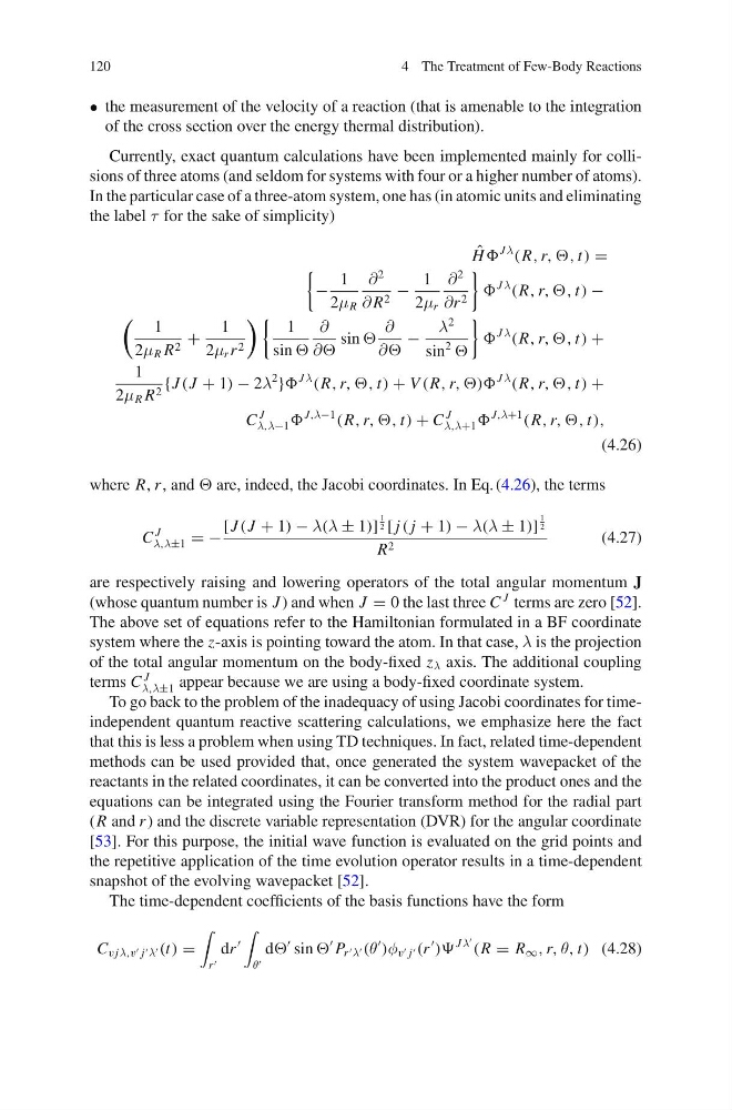
Currently, exact quantum calculations have been implemented mainly for collisions of three atoms (and seldom for systems with four or a higher number of atoms).
In the particular case of a three-atom system, one has (in atomic units and eliminating
the label τ for the sake of simplicity)
ˆ
H
J λ
(R, r, ,, t) =
−
1
2μ R
∂
2
∂ R 2 −
1
2μ r
∂
2
∂r 2
J λ
(R, r, ,, t) −
1
2μ R R 2 +
1
2μ r r 2
1
sin
∂
∂
sin
∂
∂
−
λ
2
sin
2
J λ
(R, r, ,, t) +
1
2μ R R 2 {J (J + 1) − 2λ
2
}
J λ
(R, r, ,, t) + V (R, r, ,))
J λ
(R, r, ,, t) +
C
J
λ,λ−1
J,λ−1
(R, r, ,, t) + C
J
λ,λ+1
J,λ+1
(R, r, ,, t),
(4.26)
where R, r , and are, indeed, the Jacobi coordinates. In Eq. (4.26), the terms
C
J
λ,λ±1 = −
[J (J + 1) − λ(λ ± 1)]
1
2 [ j ( j + 1) − λ(λ ± 1)]
1
2
R 2
(4.27)
are respectively raising and lowering operators of the total angular momentum J
(whose quantum number is J ) and when J = 0 the last three C
J terms are zero [52].
The above set of equations refer to the Hamiltonian formulated in a BF coordinate
system where the z-axis is pointing toward the atom. In that case, λ is the projection
of the total angular momentum on the body-fixed z λ axis. The additional coupling
terms C
J
λ,λ±1 appear because we are using a body-fixed coordinate system.
To go back to the problem of the inadequacy of using Jacobi coordinates for timeindependent quantum reactive scattering calculations, we emphasize here the fact
that this is less a problem when using TD techniques. In fact, related time-dependent
methods can be used provided that, once generated the system wavepacket of the
reactants in the related coordinates, it can be converted into the product ones and the
equations can be integrated using the Fourier transform method for the radial part
(R and r ) and the discrete variable representation (DVR) for the angular coordinate
[53]. For this purpose, the initial wave function is evaluated on the grid points and
the repetitive application of the time evolution operator results in a time-dependent
snapshot of the evolving wavepacket [52].
The time-dependent coefficients of the basis functions have the form
C v jλ,v j λ (t) =
r
dr
θ
d
sin
P r λ (θ
)φ v j (r
))
J λ
(R = R ∞ , r, θ, t) (4.28)
4 The Treatment of Few-Body Reactions
• the measurement of the velocity of a reaction (that is amenable to the integration
of the cross section over the energy thermal distribution).
Currently, exact quantum calculations have been implemented mainly for collisions of three atoms (and seldom for systems with four or a higher number of atoms).
In the particular case of a three-atom system, one has (in atomic units and eliminating
the label τ for the sake of simplicity)
ˆ
H
J λ
(R, r, ,, t) =
−
1
2μ R
∂
2
∂ R 2 −
1
2μ r
∂
2
∂r 2
J λ
(R, r, ,, t) −
1
2μ R R 2 +
1
2μ r r 2
1
sin
∂
∂
sin
∂
∂
−
λ
2
sin
2
J λ
(R, r, ,, t) +
1
2μ R R 2 {J (J + 1) − 2λ
2
}
J λ
(R, r, ,, t) + V (R, r, ,))
J λ
(R, r, ,, t) +
C
J
λ,λ−1
J,λ−1
(R, r, ,, t) + C
J
λ,λ+1
J,λ+1
(R, r, ,, t),
(4.26)
where R, r , and are, indeed, the Jacobi coordinates. In Eq. (4.26), the terms
C
J
λ,λ±1 = −
[J (J + 1) − λ(λ ± 1)]
1
2 [ j ( j + 1) − λ(λ ± 1)]
1
2
R 2
(4.27)
are respectively raising and lowering operators of the total angular momentum J
(whose quantum number is J ) and when J = 0 the last three C
J terms are zero [52].
The above set of equations refer to the Hamiltonian formulated in a BF coordinate
system where the z-axis is pointing toward the atom. In that case, λ is the projection
of the total angular momentum on the body-fixed z λ axis. The additional coupling
terms C
J
λ,λ±1 appear because we are using a body-fixed coordinate system.
To go back to the problem of the inadequacy of using Jacobi coordinates for timeindependent quantum reactive scattering calculations, we emphasize here the fact
that this is less a problem when using TD techniques. In fact, related time-dependent
methods can be used provided that, once generated the system wavepacket of the
reactants in the related coordinates, it can be converted into the product ones and the
equations can be integrated using the Fourier transform method for the radial part
(R and r ) and the discrete variable representation (DVR) for the angular coordinate
[53]. For this purpose, the initial wave function is evaluated on the grid points and
the repetitive application of the time evolution operator results in a time-dependent
snapshot of the evolving wavepacket [52].
The time-dependent coefficients of the basis functions have the form
C v jλ,v j λ (t) =
r
dr
θ
d
sin
P r λ (θ
)φ v j (r
))
J λ
(R = R ∞ , r, θ, t) (4.28)