

4.1 The Combined Dynamics of Electrons and Nuclei
113
W i = W
‡
i − W C M .
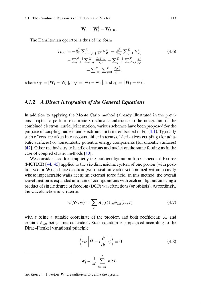
The Hamiltonian operator is thus of the form
H tot = −
2
2
N
i=1 =i‡
1
M i
∇
2
W i
−
2
2m e
K
j=1 ∇
2
w j
(4.6)
−
N −1
i=1
N
i >i
Z i Z
i q
2
e
r ii
−
K −1
j=1
K
j > j
q
2
e
r j
−
N
i=1
K
j=1
Z i q
2
e
r i j
,
where r ii = |W i − W i |, r j j =
w j − w j
, and r i j =
W i − w j
.
4.1.2 A Direct Integration of the General Equations
In addition to applying the Monte Carlo method (already illustrated in the previous chapter to perform electronic structure calculations) to the integration of the
combined electron–nuclei joint motion, various schemes have been proposed for the
purpose of coupling nuclear and electronic motions embodied in Eq. (4.1). Typically
such effects are taken into account either in terms of derivatives coupling (for adiabatic surfaces) or nonadiabatic potential energy components (for diabatic surfaces)
[42]. Other methods try to handle electrons and nuclei on the same footing as in the
case of coupled cluster methods [43].
We consider here for simplicity the multiconfiguration time-dependent Hartree
(MCTDH) [44, 45] applied to the six-dimensional system of one proton (with position vector W) and one electron (with position vector w) confined within a cavity
whose impenetrable walls act as an external force field. In this method, the overall
wavefunction is expanded as a sum of configurations with each configuration being a
product of single degree of freedom (DOF) wavefunctions (or orbitals). Accordingly,
the wavefunction is written as
ψ(W, w) =
c
A c (t)) n φ c,n (z n , t)
(4.7)
with z being a suitable coordinate of the problem and both coefficients A c and
orbitals φ c,n being time dependent. Such equation is propagated according to the
Dirac–Frenkel variational principle
δψ
ˆ
H − i
∂
∂t
ψ
= 0
(4.8)
W i =
1
M i
I
i=1 =i
M i W i
and then I − 1 vectors W i are sufficient to define the system.
113
W i = W
‡
i − W C M .
The Hamiltonian operator is thus of the form
H tot = −
2
2
N
i=1 =i‡
1
M i
∇
2
W i
−
2
2m e
K
j=1 ∇
2
w j
(4.6)
−
N −1
i=1
N
i >i
Z i Z
i q
2
e
r ii
−
K −1
j=1
K
j > j
q
2
e
r j
−
N
i=1
K
j=1
Z i q
2
e
r i j
,
where r ii = |W i − W i |, r j j =
w j − w j
, and r i j =
W i − w j
.
4.1.2 A Direct Integration of the General Equations
In addition to applying the Monte Carlo method (already illustrated in the previous chapter to perform electronic structure calculations) to the integration of the
combined electron–nuclei joint motion, various schemes have been proposed for the
purpose of coupling nuclear and electronic motions embodied in Eq. (4.1). Typically
such effects are taken into account either in terms of derivatives coupling (for adiabatic surfaces) or nonadiabatic potential energy components (for diabatic surfaces)
[42]. Other methods try to handle electrons and nuclei on the same footing as in the
case of coupled cluster methods [43].
We consider here for simplicity the multiconfiguration time-dependent Hartree
(MCTDH) [44, 45] applied to the six-dimensional system of one proton (with position vector W) and one electron (with position vector w) confined within a cavity
whose impenetrable walls act as an external force field. In this method, the overall
wavefunction is expanded as a sum of configurations with each configuration being a
product of single degree of freedom (DOF) wavefunctions (or orbitals). Accordingly,
the wavefunction is written as
ψ(W, w) =
c
A c (t)) n φ c,n (z n , t)
(4.7)
with z being a suitable coordinate of the problem and both coefficients A c and
orbitals φ c,n being time dependent. Such equation is propagated according to the
Dirac–Frenkel variational principle
δψ
ˆ
H − i
∂
∂t
ψ
= 0
(4.8)
W i =
1
M i
I
i=1 =i
M i W i
and then I − 1 vectors W i are sufficient to define the system.