

82
3 Two (or More) Magnetic Centers
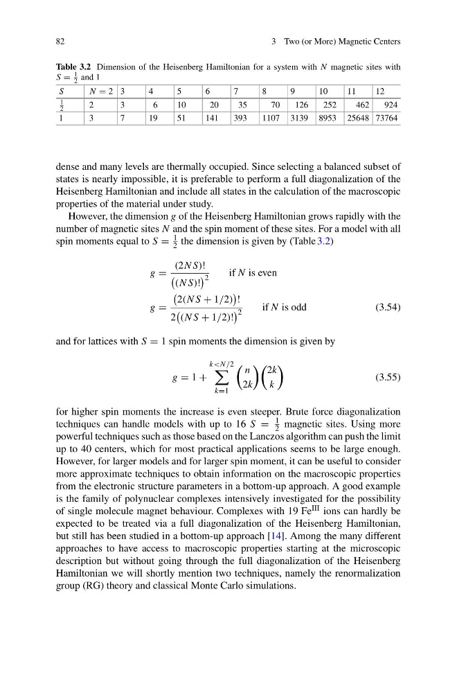
Table 3.2 Dimension of the Heisenberg Hamiltonian for a system with N magnetic sites with
S =
1
2 and 1
S
N = 2 3
4
5
6
7
8
9
10
11
12
1
2
2
3
6
10
20
35
70
126
252
462
924
1
3
7
19
51
141
393
1107 3139 8953 25648 73764
dense and many levels are thermally occupied. Since selecting a balanced subset of
states is nearly impossible, it is preferable to perform a full diagonalization of the
Heisenberg Hamiltonian and include all states in the calculation of the macroscopic
properties of the material under study.
However, the dimension g of the Heisenberg Hamiltonian grows rapidly with the
number of magnetic sites N and the spin moment of these sites. For a model with all
spin moments equal to S =
1
2 the dimension is given by (Table 3.2)
g =
(2NS)!
(NS)!
2
if N is even
g =
2(NS + 1/2)
!
2
(NS + 1/2)!
2
if N is odd
(3.54)
and for lattices with S = 1 spin moments the dimension is given by
g = 1 +
k
n
2k
2k
k
(3.55)
for higher spin moments the increase is even steeper. Brute force diagonalization
techniques can handle models with up to 16 S =
1
2 magnetic sites. Using more
powerful techniques such as those based on the Lanczos algorithm can push the limit
up to 40 centers, which for most practical applications seems to be large enough.
However, for larger models and for larger spin moment, it can be useful to consider
more approximate techniques to obtain information on the macroscopic properties
from the electronic structure parameters in a bottom-up approach. A good example
is the family of polynuclear complexes intensively investigated for the possibility
of single molecule magnet behaviour. Complexes with 19 Fe III ions can hardly be
expected to be treated via a full diagonalization of the Heisenberg Hamiltonian,
but still has been studied in a bottom-up approach [14]. Among the many different
approaches to have access to macroscopic properties starting at the microscopic
description but without going through the full diagonalization of the Heisenberg
Hamiltonian we will shortly mention two techniques, namely the renormalization
group (RG) theory and classical Monte Carlo simulations.
3 Two (or More) Magnetic Centers
Table 3.2 Dimension of the Heisenberg Hamiltonian for a system with N magnetic sites with
S =
1
2 and 1
S
N = 2 3
4
5
6
7
8
9
10
11
12
1
2
2
3
6
10
20
35
70
126
252
462
924
1
3
7
19
51
141
393
1107 3139 8953 25648 73764
dense and many levels are thermally occupied. Since selecting a balanced subset of
states is nearly impossible, it is preferable to perform a full diagonalization of the
Heisenberg Hamiltonian and include all states in the calculation of the macroscopic
properties of the material under study.
However, the dimension g of the Heisenberg Hamiltonian grows rapidly with the
number of magnetic sites N and the spin moment of these sites. For a model with all
spin moments equal to S =
1
2 the dimension is given by (Table 3.2)
g =
(2NS)!
(NS)!
2
if N is even
g =
2(NS + 1/2)
!
2
(NS + 1/2)!
2
if N is odd
(3.54)
and for lattices with S = 1 spin moments the dimension is given by
g = 1 +
k
n
2k
2k
k
(3.55)
for higher spin moments the increase is even steeper. Brute force diagonalization
techniques can handle models with up to 16 S =
1
2 magnetic sites. Using more
powerful techniques such as those based on the Lanczos algorithm can push the limit
up to 40 centers, which for most practical applications seems to be large enough.
However, for larger models and for larger spin moment, it can be useful to consider
more approximate techniques to obtain information on the macroscopic properties
from the electronic structure parameters in a bottom-up approach. A good example
is the family of polynuclear complexes intensively investigated for the possibility
of single molecule magnet behaviour. Complexes with 19 Fe III ions can hardly be
expected to be treated via a full diagonalization of the Heisenberg Hamiltonian,
but still has been studied in a bottom-up approach [14]. Among the many different
approaches to have access to macroscopic properties starting at the microscopic
description but without going through the full diagonalization of the Heisenberg
Hamiltonian we will shortly mention two techniques, namely the renormalization
group (RG) theory and classical Monte Carlo simulations.