

3.2 Model Spin Hamiltonians for Isotropic Interactions
75
−J ˆ
S z,1 ˆ
S z,2 |φ 1 φ 2 |=−
1
4
J |φ 1 φ 2 |
(3.46)
−J ˆ
S z,1 ˆ
S z,2 |φ 1 ¯
φ 2 |=
1
4
J |φ 1 ¯
φ 2 |
(3.47)
Assuming that the spatial part is identical in both functions (only spin degrees of
freedom are taken into account for the moment), the energy difference between the
two determinants gives an estimate of the magnetic coupling through E LS − E HS =
1
2 J . Here LS refers to the determinant with antiparallel alignment of the spins and HS
to the parallel alignment. This expression is easily generalized to a pair of arbitrary
spins
E LS − E HS = 2S 1 S 2 J
(3.48)
In any real case, the orbital part plays an important role and the influence of this on the
extraction of the J -value from calculations will be discussed in the next chapter. The
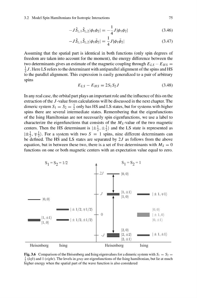
dimeric system S 1 = S 2 =
1
2 only has HS and LS states, but for systems with higher
spins there are several intermediate states. Remembering that the eigenfunctions
of the Ising Hamiltonian are not necessarily spin eigenfunctions, we use a label to
characterize the eigenfunctions that consists of the M S -value of the two magnetic
centers. Then the HS determinant is |±
1
2 , ±
1
2 and the LS state is represented as
|±
1
2 , ∓
1
2 . For a system with two S = 1 spins, nine different determinants can
be defined. The HS and LS states are separated by 2 J as follows from the above
equation, but in between these two, there is a set of five determinants with M S = 0
functions on one or both magnetic centers with an expectation value equal to zero.
Fig. 3.6 Comparison of the Heisenberg and Ising eigenvalues for a dimeric system with S 1 = S 2 =
1
2 (left)and1(right). The levels in gray are eigenfunctions of the Ising hamiltonian, but lie at much
higher energy when the spatial part of the wave function is also considered
75
−J ˆ
S z,1 ˆ
S z,2 |φ 1 φ 2 |=−
1
4
J |φ 1 φ 2 |
(3.46)
−J ˆ
S z,1 ˆ
S z,2 |φ 1 ¯
φ 2 |=
1
4
J |φ 1 ¯
φ 2 |
(3.47)
Assuming that the spatial part is identical in both functions (only spin degrees of
freedom are taken into account for the moment), the energy difference between the
two determinants gives an estimate of the magnetic coupling through E LS − E HS =
1
2 J . Here LS refers to the determinant with antiparallel alignment of the spins and HS
to the parallel alignment. This expression is easily generalized to a pair of arbitrary
spins
E LS − E HS = 2S 1 S 2 J
(3.48)
In any real case, the orbital part plays an important role and the influence of this on the
extraction of the J -value from calculations will be discussed in the next chapter. The
dimeric system S 1 = S 2 =
1
2 only has HS and LS states, but for systems with higher
spins there are several intermediate states. Remembering that the eigenfunctions
of the Ising Hamiltonian are not necessarily spin eigenfunctions, we use a label to
characterize the eigenfunctions that consists of the M S -value of the two magnetic
centers. Then the HS determinant is |±
1
2 , ±
1
2 and the LS state is represented as
|±
1
2 , ∓
1
2 . For a system with two S = 1 spins, nine different determinants can
be defined. The HS and LS states are separated by 2 J as follows from the above
equation, but in between these two, there is a set of five determinants with M S = 0
functions on one or both magnetic centers with an expectation value equal to zero.
Fig. 3.6 Comparison of the Heisenberg and Ising eigenvalues for a dimeric system with S 1 = S 2 =
1
2 (left)and1(right). The levels in gray are eigenfunctions of the Ising hamiltonian, but lie at much
higher energy when the spatial part of the wave function is also considered