

74
3 Two (or More) Magnetic Centers
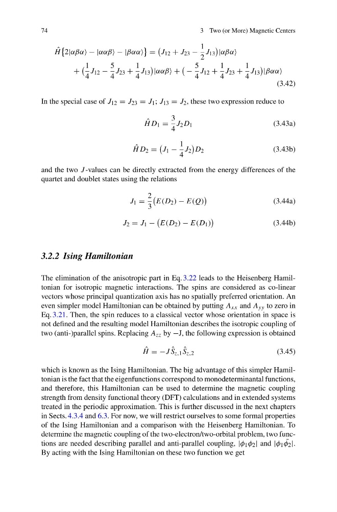
ˆ
H
2|αβα−|ααβ−|βαα
=
J 12 + J 23 −
1
2
J 13
|αβα
+
1
4
J 12 −
5
4
J 23 +
1
4
J 13
|ααβ+
−
5
4
J 12 +
1
4
J 23 +
1
4
J 13
|βαα
(3.42)
In the special case of J 12 = J 23 = J 1 ; J 13 = J 2 , these two expression reduce to
ˆ
HD 1 =
3
4
J 2 D 1
(3.43a)
ˆ
HD 2 =
J 1 −
1
4
J 2
D 2
(3.43b)
and the two J -values can be directly extracted from the energy differences of the
quartet and doublet states using the relations
J 1 =
2
3
E(D 2 ) − E(Q)
(3.44a)
J 2 = J 1 −
E(D 2 ) − E(D 1 )
(3.44b)
3.2.2 Ising Hamiltonian
The elimination of the anisotropic part in Eq. 3.22 leads to the Heisenberg Hamiltonian for isotropic magnetic interactions. The spins are considered as co-linear
vectors whose principal quantization axis has no spatially preferred orientation. An
even simpler model Hamiltonian can be obtained by putting A xx and A yy to zero in
Eq. 3.21. Then, the spin reduces to a classical vector whose orientation in space is
not defined and the resulting model Hamiltonian describes the isotropic coupling of
two (anti-)parallel spins. Replacing A zz by −J, the following expression is obtained
ˆ
H =−J ˆ
S z,1 ˆ
S z,2
(3.45)
which is known as the Ising Hamiltonian. The big advantage of this simpler Hamiltonian is the fact that the eigenfunctions correspond to monodeterminantal functions,
and therefore, this Hamiltonian can be used to determine the magnetic coupling
strength from density functional theory (DFT) calculations and in extended systems
treated in the periodic approximation. This is further discussed in the next chapters
in Sects. 4.3.4 and 6.3. For now, we will restrict ourselves to some formal properties
of the Ising Hamiltonian and a comparison with the Heisenberg Hamiltonian. To
determine the magnetic coupling of the two-electron/two-orbital problem, two functions are needed describing parallel and anti-parallel coupling, |φ 1 φ 2 | and |φ 1 ¯
φ 2 |.
By acting with the Ising Hamiltonian on these two function we get
3 Two (or More) Magnetic Centers
ˆ
H
2|αβα−|ααβ−|βαα
=
J 12 + J 23 −
1
2
J 13
|αβα
+
1
4
J 12 −
5
4
J 23 +
1
4
J 13
|ααβ+
−
5
4
J 12 +
1
4
J 23 +
1
4
J 13
|βαα
(3.42)
In the special case of J 12 = J 23 = J 1 ; J 13 = J 2 , these two expression reduce to
ˆ
HD 1 =
3
4
J 2 D 1
(3.43a)
ˆ
HD 2 =
J 1 −
1
4
J 2
D 2
(3.43b)
and the two J -values can be directly extracted from the energy differences of the
quartet and doublet states using the relations
J 1 =
2
3
E(D 2 ) − E(Q)
(3.44a)
J 2 = J 1 −
E(D 2 ) − E(D 1 )
(3.44b)
3.2.2 Ising Hamiltonian
The elimination of the anisotropic part in Eq. 3.22 leads to the Heisenberg Hamiltonian for isotropic magnetic interactions. The spins are considered as co-linear
vectors whose principal quantization axis has no spatially preferred orientation. An
even simpler model Hamiltonian can be obtained by putting A xx and A yy to zero in
Eq. 3.21. Then, the spin reduces to a classical vector whose orientation in space is
not defined and the resulting model Hamiltonian describes the isotropic coupling of
two (anti-)parallel spins. Replacing A zz by −J, the following expression is obtained
ˆ
H =−J ˆ
S z,1 ˆ
S z,2
(3.45)
which is known as the Ising Hamiltonian. The big advantage of this simpler Hamiltonian is the fact that the eigenfunctions correspond to monodeterminantal functions,
and therefore, this Hamiltonian can be used to determine the magnetic coupling
strength from density functional theory (DFT) calculations and in extended systems
treated in the periodic approximation. This is further discussed in the next chapters
in Sects. 4.3.4 and 6.3. For now, we will restrict ourselves to some formal properties
of the Ising Hamiltonian and a comparison with the Heisenberg Hamiltonian. To
determine the magnetic coupling of the two-electron/two-orbital problem, two functions are needed describing parallel and anti-parallel coupling, |φ 1 φ 2 | and |φ 1 ¯
φ 2 |.
By acting with the Ising Hamiltonian on these two function we get