

1.4 Effective Hamiltonian Theory
31
effective Hamiltonian at places where the model Hamiltonian is zero, one should
revise the expression of the model Hamiltonian. This brings us to the second type
of effective Hamiltonians that falls under the scope of this monograph; the analytical effective Hamiltonian. The above sketched procedure to derive a numerical
Hamiltonian can also be used to map the analytical expressions of a precise, but complicated model Hamiltonian onto a simpler one. In this way one can rigorously derive
new model Hamiltonians, for example when the comparison between a numerical
effective Hamiltonian and a simple model Hamiltonian fails.
Problems
1.1 Ordering by spatial or spin part. In the notation of multideterminantal wave
functions, one can either respect as much as possible the order of the spatial part in
the different determinants, or strictly maintain the order of the spin part. Construct
singlet and triplet functions for a two-electrons in two-orbitals case respecting (i) the
order of the spatial part and (ii) the order of the spin part of the total wave function.
1.2 Coulomb, exchange or other. Classify the following two-electron integrals as
Coulomb, exchange or other integral and assign a relative size (large, medium,o r
small to the integrals:
(a) φ a (1)φ b (2)|
1
r 12
|φ a (1)φ b (2)
(b)
φ a (1)φ b (1)φ a (2)φ b (2)
r 12
dτ 1 dτ 2
(c) φ a (1)φ c (2)|
1 − ˆ
P 12
r 12
|φ c (1)φ a (2)
(d) φ b (1)φ c (2)|
1
r 12
|φ c (1)φ d (2)
(e)
φ a (1)φ c (2)
1
r 12
φ c (1)φ a (2)dτ 1 dτ 2
(f)φ b (1)φ d (2)|
ˆ
P 12
r 12
|φ d (1)φ b (2)
φ a and φ b are centered on site A, φ c and φ d on site B.
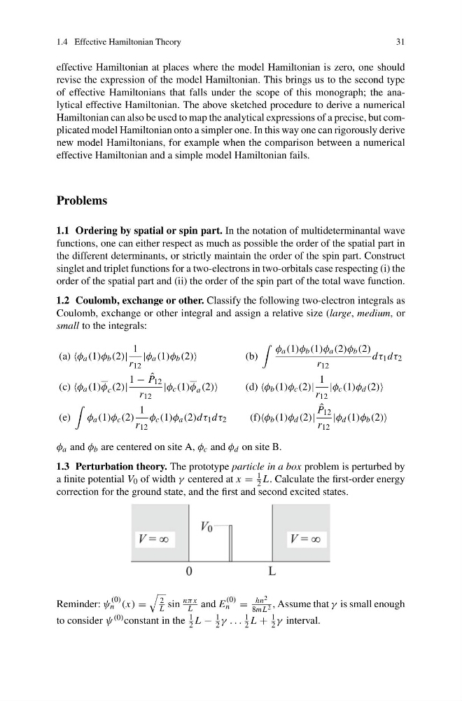
1.3 Perturbation theory. The prototype particle in a box problem is perturbed by
a finite potential V 0 of width γ centered at x =
1
2 L. Calculate the first-order energy
correction for the ground state, and the first and second excited states.
Reminder: ψ
(0)
n (x) =
2
L sin
nπ x
L and E
(0)
n =
hn 2
8mL 2 , Assume that γ is small enough
to consider ψ (0) constant in the
1
2 L −
1
2 γ...
1
2 L +
1
2 γ interval.
31
effective Hamiltonian at places where the model Hamiltonian is zero, one should
revise the expression of the model Hamiltonian. This brings us to the second type
of effective Hamiltonians that falls under the scope of this monograph; the analytical effective Hamiltonian. The above sketched procedure to derive a numerical
Hamiltonian can also be used to map the analytical expressions of a precise, but complicated model Hamiltonian onto a simpler one. In this way one can rigorously derive
new model Hamiltonians, for example when the comparison between a numerical
effective Hamiltonian and a simple model Hamiltonian fails.
Problems
1.1 Ordering by spatial or spin part. In the notation of multideterminantal wave
functions, one can either respect as much as possible the order of the spatial part in
the different determinants, or strictly maintain the order of the spin part. Construct
singlet and triplet functions for a two-electrons in two-orbitals case respecting (i) the
order of the spatial part and (ii) the order of the spin part of the total wave function.
1.2 Coulomb, exchange or other. Classify the following two-electron integrals as
Coulomb, exchange or other integral and assign a relative size (large, medium,o r
small to the integrals:
(a) φ a (1)φ b (2)|
1
r 12
|φ a (1)φ b (2)
(b)
φ a (1)φ b (1)φ a (2)φ b (2)
r 12
dτ 1 dτ 2
(c) φ a (1)φ c (2)|
1 − ˆ
P 12
r 12
|φ c (1)φ a (2)
(d) φ b (1)φ c (2)|
1
r 12
|φ c (1)φ d (2)
(e)
φ a (1)φ c (2)
1
r 12
φ c (1)φ a (2)dτ 1 dτ 2
(f)φ b (1)φ d (2)|
ˆ
P 12
r 12
|φ d (1)φ b (2)
φ a and φ b are centered on site A, φ c and φ d on site B.
1.3 Perturbation theory. The prototype particle in a box problem is perturbed by
a finite potential V 0 of width γ centered at x =
1
2 L. Calculate the first-order energy
correction for the ground state, and the first and second excited states.
Reminder: ψ
(0)
n (x) =
2
L sin
nπ x
L and E
(0)
n =
hn 2
8mL 2 , Assume that γ is small enough
to consider ψ (0) constant in the
1
2 L −
1
2 γ...
1
2 L +
1
2 γ interval.