

30
1 Basic Concepts
orthogonalization of the projections proposed by des Cloizeaux, which involves the
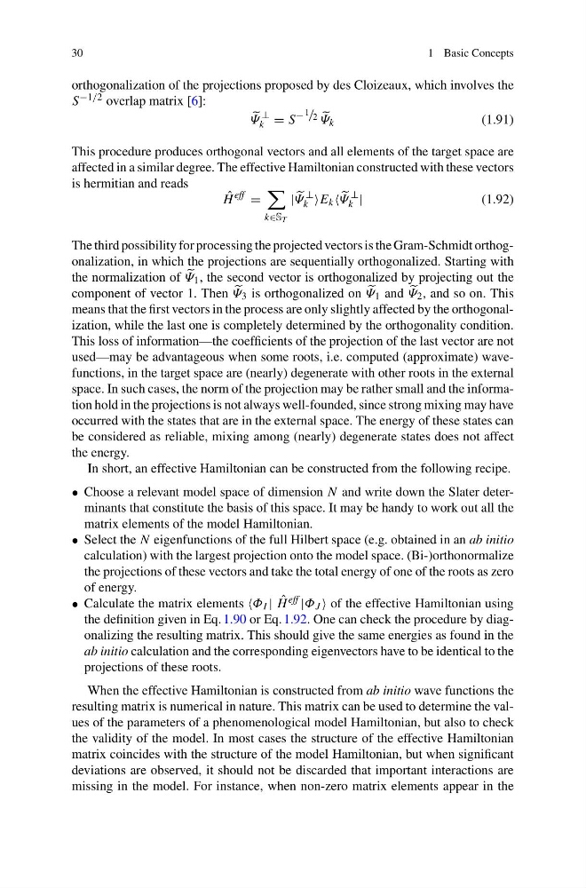
S −1/2 overlap matrix [6]:
Ψ
⊥
k = S
− 1 / 2
Ψ k
(1.91)
This procedure produces orthogonal vectors and all elements of the target space are
affected in a similar degree. The effective Hamiltonian constructed with these vectors
is hermitian and reads
ˆ
H
eff =
k∈S T
|
Ψ
⊥
k E k
Ψ
⊥
k |
(1.92)
The third possibility for processing the projected vectors is the Gram-Schmidt orthogonalization, in which the projections are sequentially orthogonalized. Starting with
the normalization of
Ψ 1 , the second vector is orthogonalized by projecting out the
component of vector 1. Then
Ψ 3 is orthogonalized on
Ψ 1 and
Ψ 2 , and so on. This
means that the first vectors in the process are only slightly affected by the orthogonalization, while the last one is completely determined by the orthogonality condition.
This loss of information—the coefficients of the projection of the last vector are not
used—may be advantageous when some roots, i.e. computed (approximate) wavefunctions, in the target space are (nearly) degenerate with other roots in the external
space. In such cases, the norm of the projection may be rather small and the information hold in the projections is not always well-founded, since strong mixing may have
occurred with the states that are in the external space. The energy of these states can
be considered as reliable, mixing among (nearly) degenerate states does not affect
the energy.
In short, an effective Hamiltonian can be constructed from the following recipe.
• Choose a relevant model space of dimension N and write down the Slater determinants that constitute the basis of this space. It may be handy to work out all the
matrix elements of the model Hamiltonian.
• Select the N eigenfunctions of the full Hilbert space (e.g. obtained in an ab initio
calculation) with the largest projection onto the model space. (Bi-)orthonormalize
the projections of these vectors and take the total energy of one of the roots as zero
of energy.
• Calculate the matrix elements Φ I | ˆ
H eff |Φ J of the effective Hamiltonian using
the definition given in Eq. 1.90 or Eq. 1.92. One can check the procedure by diagonalizing the resulting matrix. This should give the same energies as found in the
ab initio calculation and the corresponding eigenvectors have to be identical to the
projections of these roots.
When the effective Hamiltonian is constructed from ab initio wave functions the
resulting matrix is numerical in nature. This matrix can be used to determine the values of the parameters of a phenomenological model Hamiltonian, but also to check
the validity of the model. In most cases the structure of the effective Hamiltonian
matrix coincides with the structure of the model Hamiltonian, but when significant
deviations are observed, it should not be discarded that important interactions are
missing in the model. For instance, when non-zero matrix elements appear in the
1 Basic Concepts
orthogonalization of the projections proposed by des Cloizeaux, which involves the
S −1/2 overlap matrix [6]:
Ψ
⊥
k = S
− 1 / 2
Ψ k
(1.91)
This procedure produces orthogonal vectors and all elements of the target space are
affected in a similar degree. The effective Hamiltonian constructed with these vectors
is hermitian and reads
ˆ
H
eff =
k∈S T
|
Ψ
⊥
k E k
Ψ
⊥
k |
(1.92)
The third possibility for processing the projected vectors is the Gram-Schmidt orthogonalization, in which the projections are sequentially orthogonalized. Starting with
the normalization of
Ψ 1 , the second vector is orthogonalized by projecting out the
component of vector 1. Then
Ψ 3 is orthogonalized on
Ψ 1 and
Ψ 2 , and so on. This
means that the first vectors in the process are only slightly affected by the orthogonalization, while the last one is completely determined by the orthogonality condition.
This loss of information—the coefficients of the projection of the last vector are not
used—may be advantageous when some roots, i.e. computed (approximate) wavefunctions, in the target space are (nearly) degenerate with other roots in the external
space. In such cases, the norm of the projection may be rather small and the information hold in the projections is not always well-founded, since strong mixing may have
occurred with the states that are in the external space. The energy of these states can
be considered as reliable, mixing among (nearly) degenerate states does not affect
the energy.
In short, an effective Hamiltonian can be constructed from the following recipe.
• Choose a relevant model space of dimension N and write down the Slater determinants that constitute the basis of this space. It may be handy to work out all the
matrix elements of the model Hamiltonian.
• Select the N eigenfunctions of the full Hilbert space (e.g. obtained in an ab initio
calculation) with the largest projection onto the model space. (Bi-)orthonormalize
the projections of these vectors and take the total energy of one of the roots as zero
of energy.
• Calculate the matrix elements Φ I | ˆ
H eff |Φ J of the effective Hamiltonian using
the definition given in Eq. 1.90 or Eq. 1.92. One can check the procedure by diagonalizing the resulting matrix. This should give the same energies as found in the
ab initio calculation and the corresponding eigenvectors have to be identical to the
projections of these roots.
When the effective Hamiltonian is constructed from ab initio wave functions the
resulting matrix is numerical in nature. This matrix can be used to determine the values of the parameters of a phenomenological model Hamiltonian, but also to check
the validity of the model. In most cases the structure of the effective Hamiltonian
matrix coincides with the structure of the model Hamiltonian, but when significant
deviations are observed, it should not be discarded that important interactions are
missing in the model. For instance, when non-zero matrix elements appear in the