

1.4 Effective Hamiltonian Theory
29
have been put forward to interpret experimental measurements and capture the complex physics of a system in simpler concepts. The parameters of the model are usually
determined by fitting the experimental data to analytical expressions derived from
the model Hamiltonian.
In the significance used here the effective Hamiltonian maps a lengthy, highlyaccurate wave function onto a much smaller subspace in such a way that the diagonalization of the subspace gives exactly the same eigenvalues as those of the nearly exact
wave functions and the corresponding eigenvectors are projections of the original
wave functions. The dimension of the subspace is typically the same as the dimension of the space spanned by some widely used model Hamiltonian. In this way, a
one-to-one correspondence can be established between the ab initio calculations and
the model Hamiltonian. Hence, the effective Hamiltonian theory provides a rigorous
procedure to extract model parameters from accurate calculations.
Similar to what is done in QDPT, a model space S 0 of dimension N is defined as a
subspace of the full Hilbert space S of dimension M. Remember that QDPT is used
to determine accurate wave functions and energies starting from a limited description
of the system based on the model space. However, in the present case, the accurate
energies and wave functions are already known and the action goes in the opposite
direction; the lengthy wave function of length M is mapped on the smaller subspace
S 0 ensuring a minimum loss of the information contained in the full solution.
In the first place, the eigenfunctions of S (Ψ k ) have to be projected onto the model
space by applying the projection operator
ˆ
P S 0 =
N
i=1
|Φ i Φ i |
(1.87)
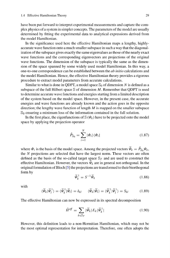
where Φ i is the basis of the model space. Among the projected vectors
Ψ k = ˆ
P S 0 Ψ k ,
the N projections are selected that have the largest norm. These vectors are often
defined as the basis of the so-called target space S T and are used to construct the
effective Hamiltonian. However, the vectors
Ψ k are in general not orthogonal. In the
original formulation of Bloch [5] the projections are transformed to their biorthogonal
form by
Ψ
†
k = S
−1
Ψ k
(1.88)
with
Ψ k |
Ψ
†
l ==
Ψ
†
k |
Ψ l =δ kl
Ψ k |
Ψ l ==
Ψ
†
k |
Ψ
†
l =S kl
(1.89)
The effective Hamiltonian can now be expressed in its spectral decomposition
ˆ
H
eff =
k∈S T
|
Ψ k E k
Ψ
†
k |
(1.90)
However, this definition leads to a non-Hermitian Hamiltonian, which may not be
the most optimal representation for interpretation. Therefore, one often adopts the
29
have been put forward to interpret experimental measurements and capture the complex physics of a system in simpler concepts. The parameters of the model are usually
determined by fitting the experimental data to analytical expressions derived from
the model Hamiltonian.
In the significance used here the effective Hamiltonian maps a lengthy, highlyaccurate wave function onto a much smaller subspace in such a way that the diagonalization of the subspace gives exactly the same eigenvalues as those of the nearly exact
wave functions and the corresponding eigenvectors are projections of the original
wave functions. The dimension of the subspace is typically the same as the dimension of the space spanned by some widely used model Hamiltonian. In this way, a
one-to-one correspondence can be established between the ab initio calculations and
the model Hamiltonian. Hence, the effective Hamiltonian theory provides a rigorous
procedure to extract model parameters from accurate calculations.
Similar to what is done in QDPT, a model space S 0 of dimension N is defined as a
subspace of the full Hilbert space S of dimension M. Remember that QDPT is used
to determine accurate wave functions and energies starting from a limited description
of the system based on the model space. However, in the present case, the accurate
energies and wave functions are already known and the action goes in the opposite
direction; the lengthy wave function of length M is mapped on the smaller subspace
S 0 ensuring a minimum loss of the information contained in the full solution.
In the first place, the eigenfunctions of S (Ψ k ) have to be projected onto the model
space by applying the projection operator
ˆ
P S 0 =
N
i=1
|Φ i Φ i |
(1.87)
where Φ i is the basis of the model space. Among the projected vectors
Ψ k = ˆ
P S 0 Ψ k ,
the N projections are selected that have the largest norm. These vectors are often
defined as the basis of the so-called target space S T and are used to construct the
effective Hamiltonian. However, the vectors
Ψ k are in general not orthogonal. In the
original formulation of Bloch [5] the projections are transformed to their biorthogonal
form by
Ψ
†
k = S
−1
Ψ k
(1.88)
with
Ψ k |
Ψ
†
l ==
Ψ
†
k |
Ψ l =δ kl
Ψ k |
Ψ l ==
Ψ
†
k |
Ψ
†
l =S kl
(1.89)
The effective Hamiltonian can now be expressed in its spectral decomposition
ˆ
H
eff =
k∈S T
|
Ψ k E k
Ψ
†
k |
(1.90)
However, this definition leads to a non-Hermitian Hamiltonian, which may not be
the most optimal representation for interpretation. Therefore, one often adopts the