

1.2 Generation of Many Electron Spin Functions
13
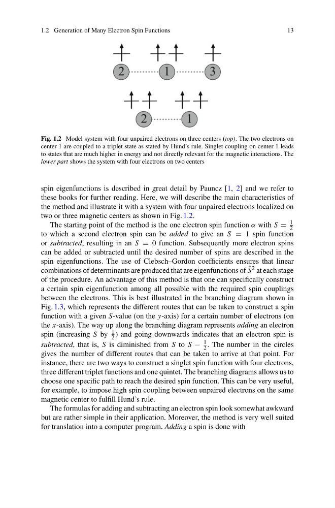
Fig. 1.2 Model system with four unpaired electrons on three centers (top). The two electrons on
center 1 are coupled to a triplet state as stated by Hund’s rule. Singlet coupling on center 1 leads
to states that are much higher in energy and not directly relevant for the magnetic interactions. The
lower part shows the system with four electrons on two centers
spin eigenfunctions is described in great detail by Pauncz [1, 2] and we refer to
these books for further reading. Here, we will describe the main characteristics of
the method and illustrate it with a system with four unpaired electrons localized on
two or three magnetic centers as shown in Fig. 1.2.
The starting point of the method is the one electron spin function α with S =
1
2
to which a second electron spin can be added to give an S = 1 spin function
or subtracted, resulting in an S = 0 function. Subsequently more electron spins
can be added or subtracted until the desired number of spins are described in the
spin eigenfunctions. The use of Clebsch–Gordon coefficients ensures that linear
combinations of determinants are produced that are eigenfunctions of ˆ
S 2 at each stage
of the procedure. An advantage of this method is that one can specifically construct
a certain spin eigenfunction among all possible with the required spin couplings
between the electrons. This is best illustrated in the branching diagram shown in
Fig. 1.3, which represents the different routes that can be taken to construct a spin
function with a given S-value (on the y-axis) for a certain number of electrons (on
the x-axis). The way up along the branching diagram represents adding an electron
spin (increasing S by
1
2 ) and going downwards indicates that an electron spin is
subtracted, that is, S is diminished from S to S −
1
2 . The number in the circles
gives the number of different routes that can be taken to arrive at that point. For
instance, there are two ways to construct a singlet spin function with four electrons,
three different triplet functions and one quintet. The branching diagrams allows us to
choose one specific path to reach the desired spin function. This can be very useful,
for example, to impose high spin coupling between unpaired electrons on the same
magnetic center to fulfill Hund’s rule.
The formulas for adding and subtracting an electron spin look somewhat awkward
but are rather simple in their application. Moreover, the method is very well suited
for translation into a computer program. Adding a spin is done with
13
Fig. 1.2 Model system with four unpaired electrons on three centers (top). The two electrons on
center 1 are coupled to a triplet state as stated by Hund’s rule. Singlet coupling on center 1 leads
to states that are much higher in energy and not directly relevant for the magnetic interactions. The
lower part shows the system with four electrons on two centers
spin eigenfunctions is described in great detail by Pauncz [1, 2] and we refer to
these books for further reading. Here, we will describe the main characteristics of
the method and illustrate it with a system with four unpaired electrons localized on
two or three magnetic centers as shown in Fig. 1.2.
The starting point of the method is the one electron spin function α with S =
1
2
to which a second electron spin can be added to give an S = 1 spin function
or subtracted, resulting in an S = 0 function. Subsequently more electron spins
can be added or subtracted until the desired number of spins are described in the
spin eigenfunctions. The use of Clebsch–Gordon coefficients ensures that linear
combinations of determinants are produced that are eigenfunctions of ˆ
S 2 at each stage
of the procedure. An advantage of this method is that one can specifically construct
a certain spin eigenfunction among all possible with the required spin couplings
between the electrons. This is best illustrated in the branching diagram shown in
Fig. 1.3, which represents the different routes that can be taken to construct a spin
function with a given S-value (on the y-axis) for a certain number of electrons (on
the x-axis). The way up along the branching diagram represents adding an electron
spin (increasing S by
1
2 ) and going downwards indicates that an electron spin is
subtracted, that is, S is diminished from S to S −
1
2 . The number in the circles
gives the number of different routes that can be taken to arrive at that point. For
instance, there are two ways to construct a singlet spin function with four electrons,
three different triplet functions and one quintet. The branching diagrams allows us to
choose one specific path to reach the desired spin function. This can be very useful,
for example, to impose high spin coupling between unpaired electrons on the same
magnetic center to fulfill Hund’s rule.
The formulas for adding and subtracting an electron spin look somewhat awkward
but are rather simple in their application. Moreover, the method is very well suited
for translation into a computer program. Adding a spin is done with