

152
5 Towards a Quantitative Understanding
Table 5.3 Decomposition of the CASPT2 contribution to the magnetic coupling in the binuclear
Cu 2+ complex with a double azido bridge
Excitation class
E (2) (singlet)
E (2) (triplet)
Difference
1h
0.000000
0.000000
0.0
1 p
0.000000
0.000000
0.0
1h-1 p
−0.017278
−0.018653
−301.8
2h
−0.000010
−0.000027
−3.9
2 p
−0.000011
−0.000031
−4.4
2h-1 p
−0.095270
−0.095938
−144.6
1h-2 p
−0.213555
−0.213649
−20.8
2h-2 p
−3.654102
−3.653976
27.5
CASPT2
−3.980233
−3.982275
−448.1 a
Energies are given in Hartree, the difference in cm −1
a The total magnetic coupling J = J [CAS(2,2)] + CASPT2 =−101.4 +−448.1 =− 549.5 cm −1
as exemplified in Table 4.1. The analysis is completely straightforward, one just has
to subtract the energy contributions of the different spin states in a class-by-class
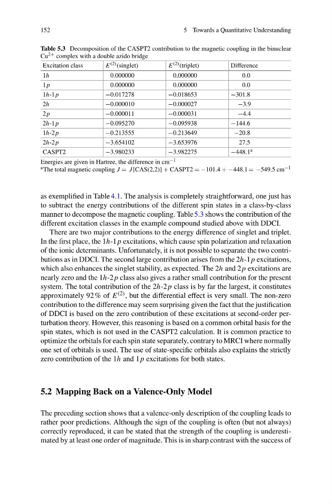
manner to decompose the magnetic coupling. Table 5.3 shows the contribution of the
different excitation classes in the example compound studied above with DDCI.
There are two major contributions to the energy difference of singlet and triplet.
In the first place, the 1h-1 p excitations, which cause spin polarization and relaxation
of the ionic determinants. Unfortunately, it is not possible to separate the two contributions as in DDCI. The second large contribution arises from the 2h-1 p excitations,
which also enhances the singlet stability, as expected. The 2h and 2 p excitations are
nearly zero and the 1h-2 p class also gives a rather small contribution for the present
system. The total contribution of the 2h-2 p class is by far the largest, it constitutes
approximately 92 % of E (2) , but the differential effect is very small. The non-zero
contribution to the difference may seem surprising given the fact that the justification
of DDCI is based on the zero contribution of these excitations at second-order perturbation theory. However, this reasoning is based on a common orbital basis for the
spin states, which is not used in the CASPT2 calculation. It is common practice to
optimize the orbitals for each spin state separately, contrary to MRCI where normally
one set of orbitals is used. The use of state-specific orbitals also explains the strictly
zero contribution of the 1h and 1 p excitations for both states.
5.2 Mapping Back on a Valence-Only Model
The preceding section shows that a valence-only description of the coupling leads to
rather poor predictions. Although the sign of the coupling is often (but not always)
correctly reproduced, it can be stated that the strength of the coupling is underestimated by at least one order of magnitude. This is in sharp contrast with the success of
5 Towards a Quantitative Understanding
Table 5.3 Decomposition of the CASPT2 contribution to the magnetic coupling in the binuclear
Cu 2+ complex with a double azido bridge
Excitation class
E (2) (singlet)
E (2) (triplet)
Difference
1h
0.000000
0.000000
0.0
1 p
0.000000
0.000000
0.0
1h-1 p
−0.017278
−0.018653
−301.8
2h
−0.000010
−0.000027
−3.9
2 p
−0.000011
−0.000031
−4.4
2h-1 p
−0.095270
−0.095938
−144.6
1h-2 p
−0.213555
−0.213649
−20.8
2h-2 p
−3.654102
−3.653976
27.5
CASPT2
−3.980233
−3.982275
−448.1 a
Energies are given in Hartree, the difference in cm −1
a The total magnetic coupling J = J [CAS(2,2)] + CASPT2 =−101.4 +−448.1 =− 549.5 cm −1
as exemplified in Table 4.1. The analysis is completely straightforward, one just has
to subtract the energy contributions of the different spin states in a class-by-class
manner to decompose the magnetic coupling. Table 5.3 shows the contribution of the
different excitation classes in the example compound studied above with DDCI.
There are two major contributions to the energy difference of singlet and triplet.
In the first place, the 1h-1 p excitations, which cause spin polarization and relaxation
of the ionic determinants. Unfortunately, it is not possible to separate the two contributions as in DDCI. The second large contribution arises from the 2h-1 p excitations,
which also enhances the singlet stability, as expected. The 2h and 2 p excitations are
nearly zero and the 1h-2 p class also gives a rather small contribution for the present
system. The total contribution of the 2h-2 p class is by far the largest, it constitutes
approximately 92 % of E (2) , but the differential effect is very small. The non-zero
contribution to the difference may seem surprising given the fact that the justification
of DDCI is based on the zero contribution of these excitations at second-order perturbation theory. However, this reasoning is based on a common orbital basis for the
spin states, which is not used in the CASPT2 calculation. It is common practice to
optimize the orbitals for each spin state separately, contrary to MRCI where normally
one set of orbitals is used. The use of state-specific orbitals also explains the strictly
zero contribution of the 1h and 1 p excitations for both states.
5.2 Mapping Back on a Valence-Only Model
The preceding section shows that a valence-only description of the coupling leads to
rather poor predictions. Although the sign of the coupling is often (but not always)
correctly reproduced, it can be stated that the strength of the coupling is underestimated by at least one order of magnitude. This is in sharp contrast with the success of