

5.1 Decomposition of the Magnetic Coupling
147
Now we replace the bare hopping matrix elements t ha and t hb by an effective parameter through
t ha t hb
∆E CT
= t
eff
ab
(5.15)
and arrive at an analytical expression for J using Eq. 3.34
J = 2K ab −
4(t
eff
ab ) 2
U
(5.16)
where the effect of the bare hopping parameter t ab has been neglected being much
smaller than t
eff
ab , which involves the bridging ligand(s). Note the similarity with the
second-order expression of Eq. 5.11. The second, antiferromagnetic term is generally
known as the kinetic exchange and is conceptually closely related to the superexchange of Anderson discussed at the end of Sect. 3.1.
5.5 Make a perturbative estimate of the contribution to J of the double LMCT
configuration with an energy of ∆E 2CT
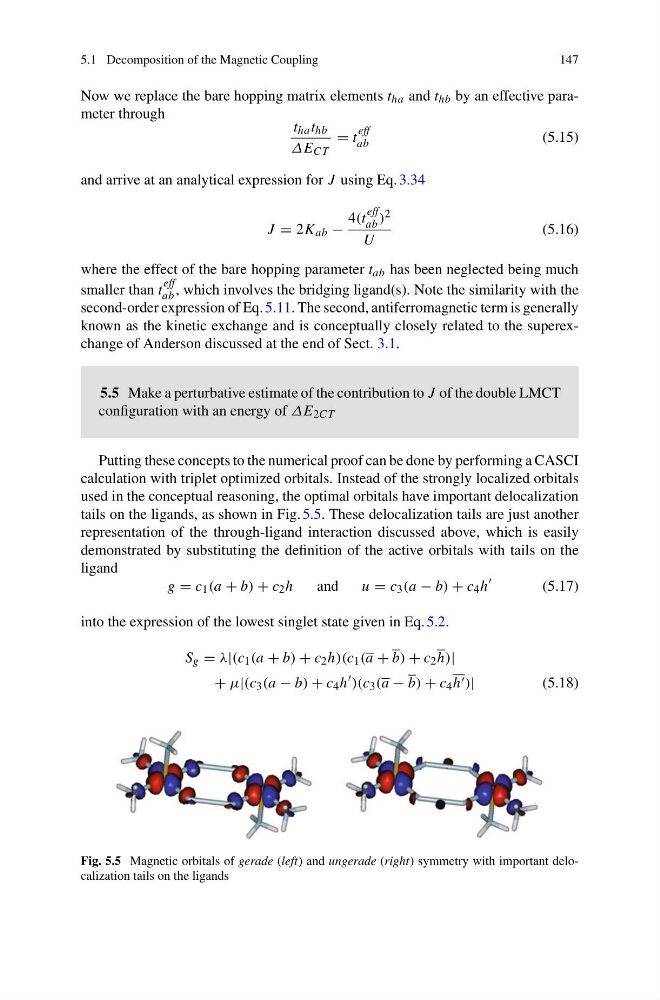
Putting these concepts to the numerical proof can be done by performing a CASCI
calculation with triplet optimized orbitals. Instead of the strongly localized orbitals
used in the conceptual reasoning, the optimal orbitals have important delocalization
tails on the ligands, as shown in Fig. 5.5. These delocalization tails are just another
representation of the through-ligand interaction discussed above, which is easily
demonstrated by substituting the definition of the active orbitals with tails on the
ligand
g = c 1 (a + b) + c 2 h
and
u = c 3 (a − b) + c 4 h
′
(5.17)
into the expression of the lowest singlet state given in Eq. 5.2.
S g = λ|(c 1 (a + b) + c 2 h)(c 1 (a + b) + c 2 h)|
+ µ|(c 3 (a − b) + c 4 h
′ )(c 3 (a − b) + c 4 h ′ )|
(5.18)
Fig. 5.5 Magnetic orbitals of gerade (left)a n dungerade (right) symmetry with important delocalization tails on the ligands
147
Now we replace the bare hopping matrix elements t ha and t hb by an effective parameter through
t ha t hb
∆E CT
= t
eff
ab
(5.15)
and arrive at an analytical expression for J using Eq. 3.34
J = 2K ab −
4(t
eff
ab ) 2
U
(5.16)
where the effect of the bare hopping parameter t ab has been neglected being much
smaller than t
eff
ab , which involves the bridging ligand(s). Note the similarity with the
second-order expression of Eq. 5.11. The second, antiferromagnetic term is generally
known as the kinetic exchange and is conceptually closely related to the superexchange of Anderson discussed at the end of Sect. 3.1.
5.5 Make a perturbative estimate of the contribution to J of the double LMCT
configuration with an energy of ∆E 2CT
Putting these concepts to the numerical proof can be done by performing a CASCI
calculation with triplet optimized orbitals. Instead of the strongly localized orbitals
used in the conceptual reasoning, the optimal orbitals have important delocalization
tails on the ligands, as shown in Fig. 5.5. These delocalization tails are just another
representation of the through-ligand interaction discussed above, which is easily
demonstrated by substituting the definition of the active orbitals with tails on the
ligand
g = c 1 (a + b) + c 2 h
and
u = c 3 (a − b) + c 4 h
′
(5.17)
into the expression of the lowest singlet state given in Eq. 5.2.
S g = λ|(c 1 (a + b) + c 2 h)(c 1 (a + b) + c 2 h)|
+ µ|(c 3 (a − b) + c 4 h
′ )(c 3 (a − b) + c 4 h ′ )|
(5.18)
Fig. 5.5 Magnetic orbitals of gerade (left)a n dungerade (right) symmetry with important delocalization tails on the ligands