

4.3 Accurate Computational Models
135
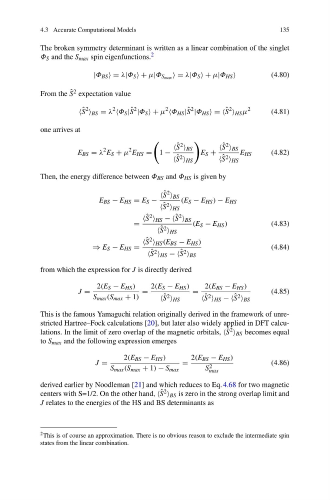
The broken symmetry determinant is written as a linear combination of the singlet
Φ S and the S max spin eigenfunctions. 2
|Φ BS =λ|Φ S +µ|Φ S max =λ|Φ S +µ|Φ HS
(4.80)
From the ˆ
S 2 expectation value
ˆ
S
2 BS = λ
2 Φ S | ˆ
S
2 |Φ S +µ
2 Φ HS | ˆ
S
2 |Φ HS == ˆ
S
2 HS µ
2
(4.81)
one arrives at
E BS = λ
2 E S + µ
2 E HS =
1 −
ˆ
S 2 BS
ˆ
S 2 HS
E S +
ˆ
S 2 BS
ˆ
S 2 HS
E HS
(4.82)
Then, the energy difference between Φ BS and Φ HS is given by
E BS − E HS = E S −
ˆ
S 2 BS
ˆ
S 2 HS
(E S − E HS ) − E HS
=
ˆ
S 2 HS −− ˆ
S 2 BS
ˆ
S 2 HS
(E S − E HS )
(4.83)
⇒ E S − E HS =
ˆ
S 2 HS (E BS − E HS )
ˆ
S 2 HS −− ˆ
S 2 BS
(4.84)
from which the expression for J is directly derived
J =
2(E S − E HS )
S max (S max + 1)
=
2(E S − E HS )
ˆ
S 2 HS
=
2(E BS − E HS )
ˆ
S 2 HS −− ˆ
S 2 BS
(4.85)
This is the famous Yamaguchi relation originally derived in the framework of unrestricted Hartree–Fock calculations [20], but later also widely applied in DFT calculations. In the limit of zero overlap of the magnetic orbitals, ˆ
S 2 BS becomes equal
to S max and the following expression emerges
J =
2(E BS − E HS )
S max (S max + 1) − S max
=
2(E BS − E HS )
S 2
max
(4.86)
derived earlier by Noodleman [21] and which reduces to Eq. 4.68 for two magnetic
centers with S=1/2. On the other hand, ˆ
S 2 BS is zero in the strong overlap limit and
J relates to the energies of the HS and BS determinants as
2 This is of course an approximation. There is no obvious reason to exclude the intermediate spin
states from the linear combination.
135
The broken symmetry determinant is written as a linear combination of the singlet
Φ S and the S max spin eigenfunctions. 2
|Φ BS =λ|Φ S +µ|Φ S max =λ|Φ S +µ|Φ HS
(4.80)
From the ˆ
S 2 expectation value
ˆ
S
2 BS = λ
2 Φ S | ˆ
S
2 |Φ S +µ
2 Φ HS | ˆ
S
2 |Φ HS == ˆ
S
2 HS µ
2
(4.81)
one arrives at
E BS = λ
2 E S + µ
2 E HS =
1 −
ˆ
S 2 BS
ˆ
S 2 HS
E S +
ˆ
S 2 BS
ˆ
S 2 HS
E HS
(4.82)
Then, the energy difference between Φ BS and Φ HS is given by
E BS − E HS = E S −
ˆ
S 2 BS
ˆ
S 2 HS
(E S − E HS ) − E HS
=
ˆ
S 2 HS −− ˆ
S 2 BS
ˆ
S 2 HS
(E S − E HS )
(4.83)
⇒ E S − E HS =
ˆ
S 2 HS (E BS − E HS )
ˆ
S 2 HS −− ˆ
S 2 BS
(4.84)
from which the expression for J is directly derived
J =
2(E S − E HS )
S max (S max + 1)
=
2(E S − E HS )
ˆ
S 2 HS
=
2(E BS − E HS )
ˆ
S 2 HS −− ˆ
S 2 BS
(4.85)
This is the famous Yamaguchi relation originally derived in the framework of unrestricted Hartree–Fock calculations [20], but later also widely applied in DFT calculations. In the limit of zero overlap of the magnetic orbitals, ˆ
S 2 BS becomes equal
to S max and the following expression emerges
J =
2(E BS − E HS )
S max (S max + 1) − S max
=
2(E BS − E HS )
S 2
max
(4.86)
derived earlier by Noodleman [21] and which reduces to Eq. 4.68 for two magnetic
centers with S=1/2. On the other hand, ˆ
S 2 BS is zero in the strong overlap limit and
J relates to the energies of the HS and BS determinants as
2 This is of course an approximation. There is no obvious reason to exclude the intermediate spin
states from the linear combination.