

4.3 Accurate Computational Models
133
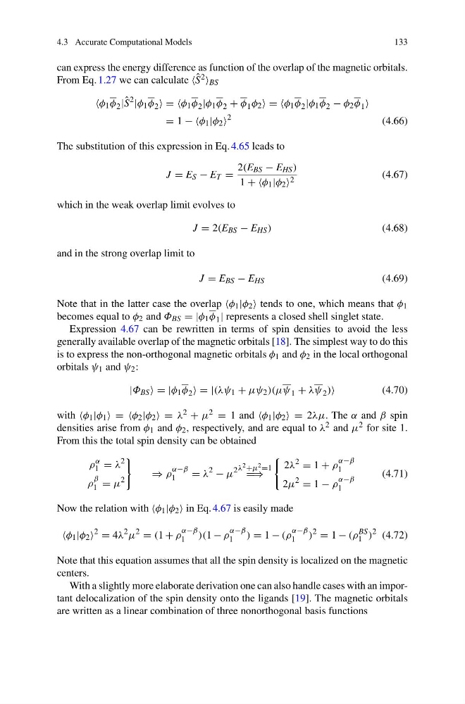
can express the energy difference as function of the overlap of the magnetic orbitals.
From Eq. 1.27 we can calculate ˆ
S 2 BS
φ 1 φ 2 | ˆ
S
2 |φ 1 φ 2 ==φ 1 φ 2 |φ 1 φ 2 + φ 1 φ 2 ==φ 1 φ 2 |φ 1 φ 2 − φ 2 φ 1
= 1 −−φ 1 |φ 2
2
(4.66)
The substitution of this expression in Eq. 4.65 leads to
J = E S − E T =
2(E BS − E HS )
1 ++φ 1 |φ 2 2
(4.67)
which in the weak overlap limit evolves to
J = 2(E BS − E HS )
(4.68)
and in the strong overlap limit to
J = E BS − E HS
(4.69)
Note that in the latter case the overlap φ 1 |φ 2 tends to one, which means that φ 1
becomes equal to φ 2 and Φ BS =|φ 1 φ 1 | represents a closed shell singlet state.
Expression 4.67 can be rewritten in terms of spin densities to avoid the less
generally available overlap of the magnetic orbitals [18]. The simplest way to do this
is to express the non-orthogonal magnetic orbitals φ 1 and φ 2 in the local orthogonal
orbitals ψ 1 and ψ 2 :
|Φ BS =|φ 1 φ 2 =|(λψ 1 + µψ 2 )(µψ 1 + λψ 2 )
(4.70)
with φ 1 |φ 1 == φ 2 |φ 2 =λ 2 + µ 2 = 1 and φ 1 |φ 2 =2λµ.T h eα and β spin
densities arise from φ 1 and φ 2 , respectively, and are equal to λ 2 and µ 2 for site 1.
From this the total spin density can be obtained
ρ
α
1 = λ
2
ρ
β
1 = µ
2
⇒ ρ
α−β
1
= λ
2 − µ
2 λ 2 +µ 2 =1
=⇒
2λ
2 = 1 + ρ
α−β
1
2µ
2 = 1 − ρ
α−β
1
(4.71)
Now the relation with φ 1 |φ 2 in Eq. 4.67 is easily made
φ 1 |φ 2
2 = 4λ
2 µ
2 = (1 + ρ
α−β
1
)(1 − ρ
α−β
1
) = 1 − (ρ
α−β
1
)
2 = 1 − (ρ
BS
1 )
2 (4.72)
Note that this equation assumes that all the spin density is localized on the magnetic
centers.
With a slightly more elaborate derivation one can also handle cases with an important delocalization of the spin density onto the ligands [19]. The magnetic orbitals
are written as a linear combination of three nonorthogonal basis functions
133
can express the energy difference as function of the overlap of the magnetic orbitals.
From Eq. 1.27 we can calculate ˆ
S 2 BS
φ 1 φ 2 | ˆ
S
2 |φ 1 φ 2 ==φ 1 φ 2 |φ 1 φ 2 + φ 1 φ 2 ==φ 1 φ 2 |φ 1 φ 2 − φ 2 φ 1
= 1 −−φ 1 |φ 2
2
(4.66)
The substitution of this expression in Eq. 4.65 leads to
J = E S − E T =
2(E BS − E HS )
1 ++φ 1 |φ 2 2
(4.67)
which in the weak overlap limit evolves to
J = 2(E BS − E HS )
(4.68)
and in the strong overlap limit to
J = E BS − E HS
(4.69)
Note that in the latter case the overlap φ 1 |φ 2 tends to one, which means that φ 1
becomes equal to φ 2 and Φ BS =|φ 1 φ 1 | represents a closed shell singlet state.
Expression 4.67 can be rewritten in terms of spin densities to avoid the less
generally available overlap of the magnetic orbitals [18]. The simplest way to do this
is to express the non-orthogonal magnetic orbitals φ 1 and φ 2 in the local orthogonal
orbitals ψ 1 and ψ 2 :
|Φ BS =|φ 1 φ 2 =|(λψ 1 + µψ 2 )(µψ 1 + λψ 2 )
(4.70)
with φ 1 |φ 1 == φ 2 |φ 2 =λ 2 + µ 2 = 1 and φ 1 |φ 2 =2λµ.T h eα and β spin
densities arise from φ 1 and φ 2 , respectively, and are equal to λ 2 and µ 2 for site 1.
From this the total spin density can be obtained
ρ
α
1 = λ
2
ρ
β
1 = µ
2
⇒ ρ
α−β
1
= λ
2 − µ
2 λ 2 +µ 2 =1
=⇒
2λ
2 = 1 + ρ
α−β
1
2µ
2 = 1 − ρ
α−β
1
(4.71)
Now the relation with φ 1 |φ 2 in Eq. 4.67 is easily made
φ 1 |φ 2
2 = 4λ
2 µ
2 = (1 + ρ
α−β
1
)(1 − ρ
α−β
1
) = 1 − (ρ
α−β
1
)
2 = 1 − (ρ
BS
1 )
2 (4.72)
Note that this equation assumes that all the spin density is localized on the magnetic
centers.
With a slightly more elaborate derivation one can also handle cases with an important delocalization of the spin density onto the ligands [19]. The magnetic orbitals
are written as a linear combination of three nonorthogonal basis functions