

114
4 From Orbital Models to Accurate Predictions
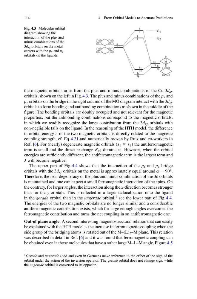
Fig. 4.3 Molecular orbital
diagram showing the
interaction of the plus and
minus combinations of the
3d xy orbitals on the metal
centers with the p x and p y
orbitals on the ligands
the magnetic orbitals arise from the plus and minus combinations of the Cu-3d xy
orbitals, shown on the left in Fig. 4.3. The plus and minus combinations of the p x and
p y orbitals on the bridge in the right column of the MO diagram interact with the 3d xy
orbitals to form bonding and antibonding combinations as shown in the middle of the
figure. The bonding orbitals are doubly occupied and not relevant for the magnetic
properties, but the antibonding combinations correspond to the magnetic orbitals,
in which we readily recognize the large contribution from the 3d xy orbitals with
non-negligible tails on the ligand. In the reasoning of the HTH model, the difference
in orbital energy ε of the two magnetic orbitals is directly related to the magnetic
coupling strength, cf. Eq. 4.21 and numerically proven by Ruiz and co-workers in
Ref. [6]. For (nearly) degenerate magnetic orbitals (ε 1 ≈ ε 2 ) the antiferromagnetic
term is small and the direct exchange K ab dominates. However, when the orbital
energies are sufficiently different, the antiferromagnetic term is the largest term and
J will become negative.
The upper part of Fig. 4.4 shows that the interaction of the p x and p y bridge
orbitals with the 3d xy orbitals on the metal is approximately equal around α = 90 ◦ .
Therefore, the near degeneracy of the plus and minus combination of the 3d orbitals
is maintained and one can expect a small ferromagnetic interaction of the spins. On
the contrary, for larger angles, the interaction along the x-direction becomes stronger
than for the y orbitals. This is reflected in a larger delocalization onto the ligand
in the gerade orbital than in the ungerade orbital, 1 see the lower part of Fig. 4.4.
The energies of the two magnetic orbitals are no longer similar and a considerable
antiferromagnetic contribution exists, which for large enough angles overcomes the
ferromagnetic contribution and turns the net coupling in an antiferromagnetic one.
Out-of plane angle: A second interesting magnetostructural relation that can easily
be explained with the HTH model is the increase in ferromagnetic coupling when the
side group of the bridging atoms is rotated out of the M–(L) 2 –M plane. This relation
was described in detail in Ref. [6] and it was found that ferromagnetic coupling can
be obtained even in those molecules that have a rather large M–L–M angle. Figure 4.5
1 Gerade and ungerade (odd and even in German) make reference to the effect of the sign of the
orbital under the action of the inversion operator. The gerade orbital does not change sign, while
the ungerade orbital is converted to its opposite.
4 From Orbital Models to Accurate Predictions
Fig. 4.3 Molecular orbital
diagram showing the
interaction of the plus and
minus combinations of the
3d xy orbitals on the metal
centers with the p x and p y
orbitals on the ligands
the magnetic orbitals arise from the plus and minus combinations of the Cu-3d xy
orbitals, shown on the left in Fig. 4.3. The plus and minus combinations of the p x and
p y orbitals on the bridge in the right column of the MO diagram interact with the 3d xy
orbitals to form bonding and antibonding combinations as shown in the middle of the
figure. The bonding orbitals are doubly occupied and not relevant for the magnetic
properties, but the antibonding combinations correspond to the magnetic orbitals,
in which we readily recognize the large contribution from the 3d xy orbitals with
non-negligible tails on the ligand. In the reasoning of the HTH model, the difference
in orbital energy ε of the two magnetic orbitals is directly related to the magnetic
coupling strength, cf. Eq. 4.21 and numerically proven by Ruiz and co-workers in
Ref. [6]. For (nearly) degenerate magnetic orbitals (ε 1 ≈ ε 2 ) the antiferromagnetic
term is small and the direct exchange K ab dominates. However, when the orbital
energies are sufficiently different, the antiferromagnetic term is the largest term and
J will become negative.
The upper part of Fig. 4.4 shows that the interaction of the p x and p y bridge
orbitals with the 3d xy orbitals on the metal is approximately equal around α = 90 ◦ .
Therefore, the near degeneracy of the plus and minus combination of the 3d orbitals
is maintained and one can expect a small ferromagnetic interaction of the spins. On
the contrary, for larger angles, the interaction along the x-direction becomes stronger
than for the y orbitals. This is reflected in a larger delocalization onto the ligand
in the gerade orbital than in the ungerade orbital, 1 see the lower part of Fig. 4.4.
The energies of the two magnetic orbitals are no longer similar and a considerable
antiferromagnetic contribution exists, which for large enough angles overcomes the
ferromagnetic contribution and turns the net coupling in an antiferromagnetic one.
Out-of plane angle: A second interesting magnetostructural relation that can easily
be explained with the HTH model is the increase in ferromagnetic coupling when the
side group of the bridging atoms is rotated out of the M–(L) 2 –M plane. This relation
was described in detail in Ref. [6] and it was found that ferromagnetic coupling can
be obtained even in those molecules that have a rather large M–L–M angle. Figure 4.5
1 Gerade and ungerade (odd and even in German) make reference to the effect of the sign of the
orbital under the action of the inversion operator. The gerade orbital does not change sign, while
the ungerade orbital is converted to its opposite.