

4.2 Magnetostructural Correlations
113
4.2 Magnetostructural Correlations
From the very beginning of the study of the magnetic interactions in transition metal
complexes a large part of the effort has been dedicated to derive relations between the
geometrical structure of the complex and the nature and magnitude of the coupling of
the localized spin moments. These magnetostructural correlations can be extremely
useful to rationalize the variations in the magnetic behaviour of a family of similar
complexes or to design new complexes with the desired properties. Magnetostructural
relations can be extracted from experimental studies by comparing a large group of
compounds and relate geometric parameters with the observed magnetic behaviour.
This requires a large set of data, but it is often difficult to separate different (opposing)
effects. On the other hand, theoretical studies can take a (model) complex and modify
the geometry at will to establish the influence of a certain geometric parameter on the
magnetic interaction. Combined with the qualitative valence-only models discussed
in the previous sections one can boil down the complicated magnetic behaviour
to very simple concepts and straightforward magnetostructural correlations. These
concepts and correlations can yield design rules that can be utilized in the synthesis
of materials with pre-defined magnetic properties.
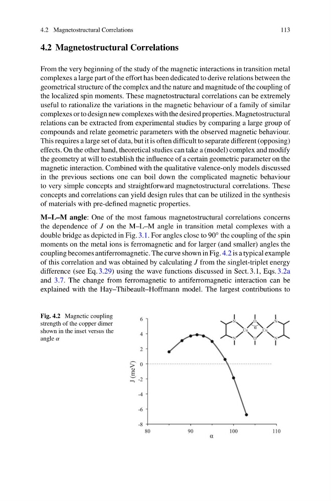
M–L–M angle: One of the most famous magnetostructural correlations concerns
the dependence of J on the M–L–M angle in transition metal complexes with a
double bridge as depicted in Fig. 3.1. For angles close to 90 ◦ the coupling of the spin
moments on the metal ions is ferromagnetic and for larger (and smaller) angles the
coupling becomes antiferromagnetic. The curve shown in Fig. 4.2 is a typical example
of this correlation and was obtained by calculating J from the singlet-triplet energy
difference (see Eq. 3.29) using the wave functions discussed in Sect. 3.1, Eqs. 3.2a
and 3.7. The change from ferromagnetic to antiferromagnetic interaction can be
explained with the Hay–Thibeault–Hoffmann model. The largest contributions to
Fig. 4.2 Magnetic coupling
strength of the copper dimer
shown in the inset versus the
angle α
113
4.2 Magnetostructural Correlations
From the very beginning of the study of the magnetic interactions in transition metal
complexes a large part of the effort has been dedicated to derive relations between the
geometrical structure of the complex and the nature and magnitude of the coupling of
the localized spin moments. These magnetostructural correlations can be extremely
useful to rationalize the variations in the magnetic behaviour of a family of similar
complexes or to design new complexes with the desired properties. Magnetostructural
relations can be extracted from experimental studies by comparing a large group of
compounds and relate geometric parameters with the observed magnetic behaviour.
This requires a large set of data, but it is often difficult to separate different (opposing)
effects. On the other hand, theoretical studies can take a (model) complex and modify
the geometry at will to establish the influence of a certain geometric parameter on the
magnetic interaction. Combined with the qualitative valence-only models discussed
in the previous sections one can boil down the complicated magnetic behaviour
to very simple concepts and straightforward magnetostructural correlations. These
concepts and correlations can yield design rules that can be utilized in the synthesis
of materials with pre-defined magnetic properties.
M–L–M angle: One of the most famous magnetostructural correlations concerns
the dependence of J on the M–L–M angle in transition metal complexes with a
double bridge as depicted in Fig. 3.1. For angles close to 90 ◦ the coupling of the spin
moments on the metal ions is ferromagnetic and for larger (and smaller) angles the
coupling becomes antiferromagnetic. The curve shown in Fig. 4.2 is a typical example
of this correlation and was obtained by calculating J from the singlet-triplet energy
difference (see Eq. 3.29) using the wave functions discussed in Sect. 3.1, Eqs. 3.2a
and 3.7. The change from ferromagnetic to antiferromagnetic interaction can be
explained with the Hay–Thibeault–Hoffmann model. The largest contributions to
Fig. 4.2 Magnetic coupling
strength of the copper dimer
shown in the inset versus the
angle α