

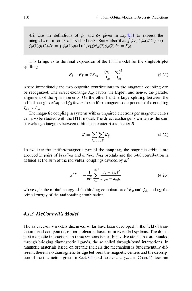
110
4 From Orbital Models to Accurate Predictions
4.2 Use the definitions of φ 1 and φ 2 given in Eq. 4.11 to express the
integral J 11 in terms of local orbitals. Remember that
φ a (1)φ a (2)(1/r 12 )
φ b (1)φ b (2)dτ =
φ a (1)φ b (1)(1/r 12 )φ a (2)φ b (2)dτ = K ab .
This brings us to the final expression of the HTH model for the singlet-triplet
splitting
E S − E T = 2K ab −
(ε 1 − ε 2 ) 2
J aa − J ab
(4.21)
where immediately the two opposite contributions to the magnetic coupling can
be recognized. The direct exchange K ab favors the triplet, and hence, the parallel
alignment of the spin moments. On the other hand, a large splitting between the
orbital energies of φ 1 and φ 2 favors the antiferromagnetic component of the coupling
J aa > J ab .
The magnetic coupling in systems with m unpaired electrons per magnetic center
can also be studied with the HTH model. The direct exchange is written as the sum
of exchange integrals between orbitals on center A and center B
K =
i∈A
j∈B
K ij
(4.22)
To evaluate the antiferromagnetic part of the coupling, the magnetic orbitals are
grouped in pairs of bonding and antibonding orbitals and the total contribution is
defined as the sum of the individual couplings divided by m 2
J
AF =−
1
m 2
m/2
i=1
(ε i − ε 2i ) 2
J a i a i − J a i b i
(4.23)
where ε i is the orbital energy of the binding combination of ψ a and ψ b , and ε 2i the
orbital energy of the antibonding combination.
4.1.3 McConnell’s Model
The valence-only models discussed so far have been developed in the field of transition metal compounds, either molecular based or in extended systems. The dominant magnetic interactions in these systems typically involve atoms that are bonded
through bridging diamagnetic ligands, the so-called through-bond interactions. In
magnetic materials based on organic radicals the mechanism is fundamentally different; there is no diamagnetic bridge between the magnetic centers and the description of the interaction given in Sect. 3.1 (and further analyzed in Chap. 5) does not
4 From Orbital Models to Accurate Predictions
4.2 Use the definitions of φ 1 and φ 2 given in Eq. 4.11 to express the
integral J 11 in terms of local orbitals. Remember that
φ a (1)φ a (2)(1/r 12 )
φ b (1)φ b (2)dτ =
φ a (1)φ b (1)(1/r 12 )φ a (2)φ b (2)dτ = K ab .
This brings us to the final expression of the HTH model for the singlet-triplet
splitting
E S − E T = 2K ab −
(ε 1 − ε 2 ) 2
J aa − J ab
(4.21)
where immediately the two opposite contributions to the magnetic coupling can
be recognized. The direct exchange K ab favors the triplet, and hence, the parallel
alignment of the spin moments. On the other hand, a large splitting between the
orbital energies of φ 1 and φ 2 favors the antiferromagnetic component of the coupling
J aa > J ab .
The magnetic coupling in systems with m unpaired electrons per magnetic center
can also be studied with the HTH model. The direct exchange is written as the sum
of exchange integrals between orbitals on center A and center B
K =
i∈A
j∈B
K ij
(4.22)
To evaluate the antiferromagnetic part of the coupling, the magnetic orbitals are
grouped in pairs of bonding and antibonding orbitals and the total contribution is
defined as the sum of the individual couplings divided by m 2
J
AF =−
1
m 2
m/2
i=1
(ε i − ε 2i ) 2
J a i a i − J a i b i
(4.23)
where ε i is the orbital energy of the binding combination of ψ a and ψ b , and ε 2i the
orbital energy of the antibonding combination.
4.1.3 McConnell’s Model
The valence-only models discussed so far have been developed in the field of transition metal compounds, either molecular based or in extended systems. The dominant magnetic interactions in these systems typically involve atoms that are bonded
through bridging diamagnetic ligands, the so-called through-bond interactions. In
magnetic materials based on organic radicals the mechanism is fundamentally different; there is no diamagnetic bridge between the magnetic centers and the description of the interaction given in Sect. 3.1 (and further analyzed in Chap. 5) does not