

3.4 Complex Interactions
99
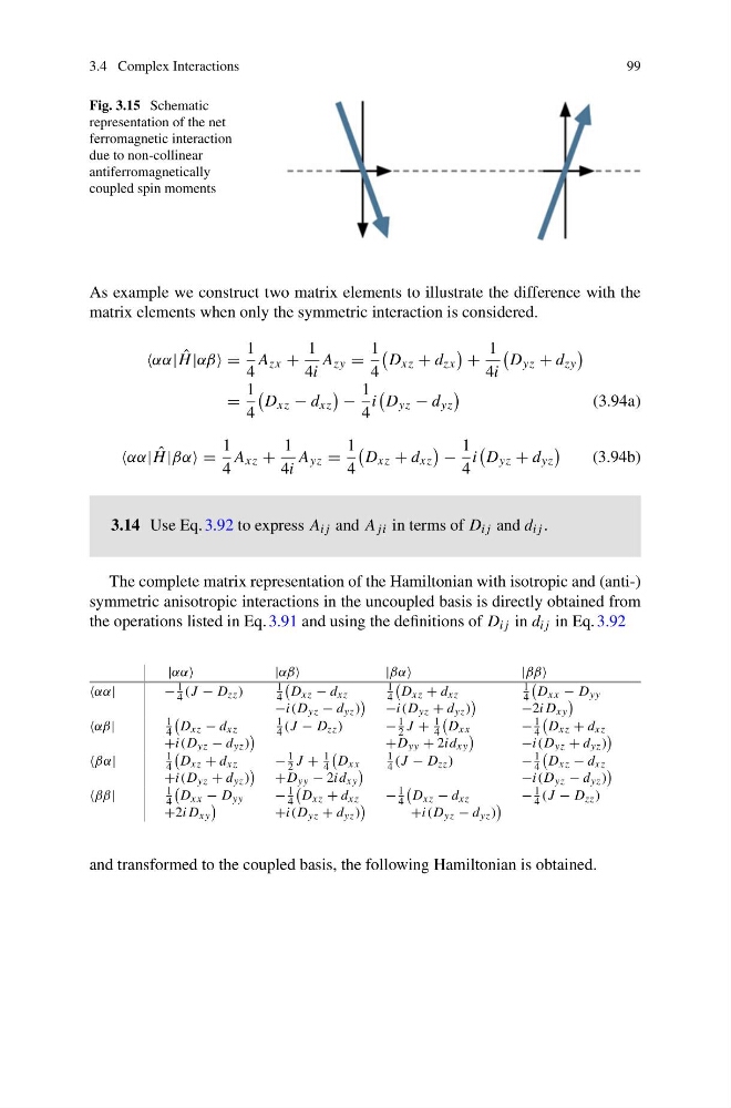
Fig. 3.15 Schematic
representation of the net
ferromagnetic interaction
due to non-collinear
antiferromagnetically
coupled spin moments
As example we construct two matrix elements to illustrate the difference with the
matrix elements when only the symmetric interaction is considered.
αα| ˆ
H |αβ =
1
4
A zx +
1
4i
A zy =
1
4
D xz + d zx
+
1
4i
D yz + d zy
=
1
4
D xz − d xz
−
1
4
i
D yz − d yz
(3.94a)
αα| ˆ
H |βα=
1
4
A xz +
1
4i
A yz =
1
4
D xz + d xz
−
1
4
i
D yz + d yz
(3.94b)
3.14 Use Eq. 3.92 to express A ij and A ji in terms of D ij and d ij .
The complete matrix representation of the Hamiltonian with isotropic and (anti-)
symmetric anisotropic interactions in the uncoupled basis is directly obtained from
the operations listed in Eq. 3.91 and using the definitions of D ij in d ij in Eq. 3.92
|αα| αβ| βα| ββ
αα|
−
1
4 (J − D zz )
1
4
D xz − d xz
1
4
D xz + d xz
1
4
D xx − D yy
−i(D yz − d yz )
−i(D yz + d yz )
−2iD xy
αβ |
1
4
D xz − d xz
1
4 (J − D zz )
−
1
2 J +
1
4
D xx
−
1
4
D xz + d xz
+i(D yz − d yz )
+D yy + 2id xy
−i(D yz + d yz )
βα|
1
4
D xz + d xz
−
1
2 J +
1
4
D xx
1
4 (J − D zz )
−
1
4
D xz − d xz
+i(D yz + d yz )
+D yy − 2id xy
−i(D yz − d yz )
ββ|
1
4
D xx − D yy
−
1
4
D xz + d xz
−
1
4
D xz − d xz
−
1
4 (J − D zz )
+2iD xy
+i(D yz + d yz )
+i(D yz − d yz )
and transformed to the coupled basis, the following Hamiltonian is obtained.
99
Fig. 3.15 Schematic
representation of the net
ferromagnetic interaction
due to non-collinear
antiferromagnetically
coupled spin moments
As example we construct two matrix elements to illustrate the difference with the
matrix elements when only the symmetric interaction is considered.
αα| ˆ
H |αβ =
1
4
A zx +
1
4i
A zy =
1
4
D xz + d zx
+
1
4i
D yz + d zy
=
1
4
D xz − d xz
−
1
4
i
D yz − d yz
(3.94a)
αα| ˆ
H |βα=
1
4
A xz +
1
4i
A yz =
1
4
D xz + d xz
−
1
4
i
D yz + d yz
(3.94b)
3.14 Use Eq. 3.92 to express A ij and A ji in terms of D ij and d ij .
The complete matrix representation of the Hamiltonian with isotropic and (anti-)
symmetric anisotropic interactions in the uncoupled basis is directly obtained from
the operations listed in Eq. 3.91 and using the definitions of D ij in d ij in Eq. 3.92
|αα| αβ| βα| ββ
αα|
−
1
4 (J − D zz )
1
4
D xz − d xz
1
4
D xz + d xz
1
4
D xx − D yy
−i(D yz − d yz )
−i(D yz + d yz )
−2iD xy
αβ |
1
4
D xz − d xz
1
4 (J − D zz )
−
1
2 J +
1
4
D xx
−
1
4
D xz + d xz
+i(D yz − d yz )
+D yy + 2id xy
−i(D yz + d yz )
βα|
1
4
D xz + d xz
−
1
2 J +
1
4
D xx
1
4 (J − D zz )
−
1
4
D xz − d xz
+i(D yz + d yz )
+D yy − 2id xy
−i(D yz − d yz )
ββ|
1
4
D xx − D yy
−
1
4
D xz + d xz
−
1
4
D xz − d xz
−
1
4 (J − D zz )
+2iD xy
+i(D yz + d yz )
+i(D yz − d yz )
and transformed to the coupled basis, the following Hamiltonian is obtained.