

3.3 From Micro to Macro: The Bottom-Up Approach
87
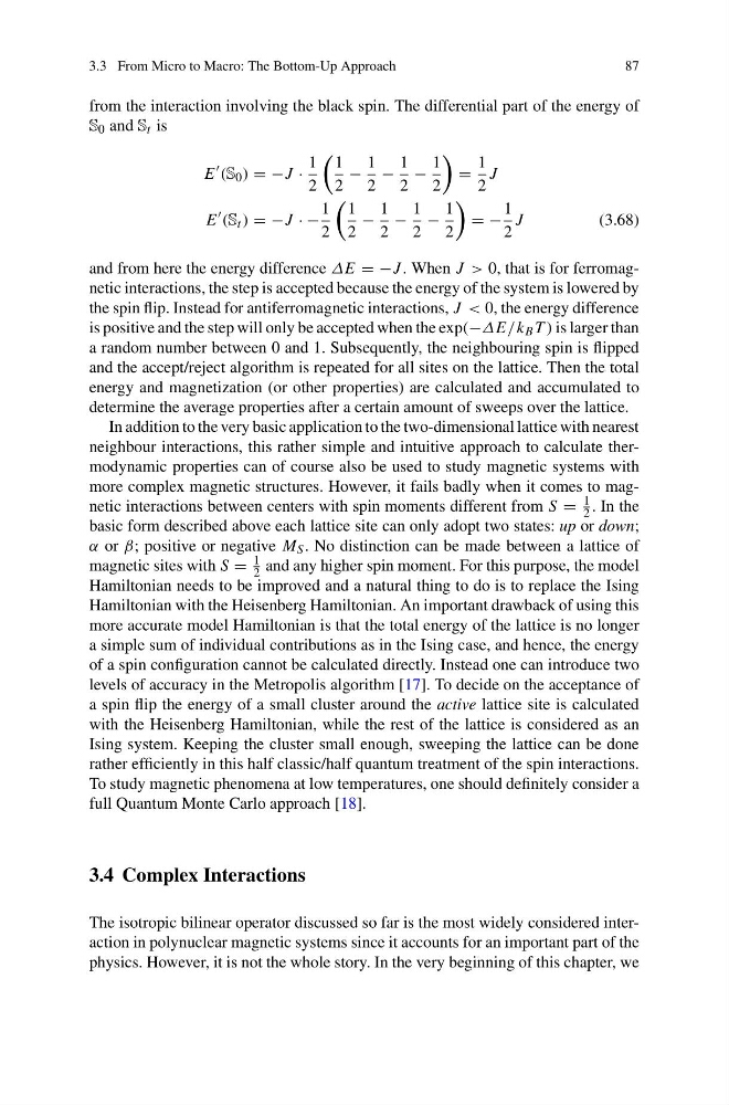
from the interaction involving the black spin. The differential part of the energy of
S 0 and S t is
E
′ (S 0 ) =−J ·
1
2
1
2
−
1
2
−
1
2
−
1
2
=
1
2
J
E
′ (S t ) =−J ·−
1
2
1
2
−
1
2
−
1
2
−
1
2
=−
1
2
J
(3.68)
and from here the energy difference ∆E =−J . When J > 0, that is for ferromagnetic interactions, the step is accepted because the energy of the system is lowered by
the spin flip. Instead for antiferromagnetic interactions, J < 0, the energy difference
is positive and the step will only be accepted when the exp(−∆E/k B T ) is larger than
a random number between 0 and 1. Subsequently, the neighbouring spin is flipped
and the accept/reject algorithm is repeated for all sites on the lattice. Then the total
energy and magnetization (or other properties) are calculated and accumulated to
determine the average properties after a certain amount of sweeps over the lattice.
In addition to the very basic application to the two-dimensional lattice with nearest
neighbour interactions, this rather simple and intuitive approach to calculate thermodynamic properties can of course also be used to study magnetic systems with
more complex magnetic structures. However, it fails badly when it comes to magnetic interactions between centers with spin moments different from S =
1
2 .Inthe
basic form described above each lattice site can only adopt two states: up or down;
α or β; positive or negative M S . No distinction can be made between a lattice of
magnetic sites with S =
1
2 and any higher spin moment. For this purpose, the model
Hamiltonian needs to be improved and a natural thing to do is to replace the Ising
Hamiltonian with the Heisenberg Hamiltonian. An important drawback of using this
more accurate model Hamiltonian is that the total energy of the lattice is no longer
a simple sum of individual contributions as in the Ising case, and hence, the energy
of a spin configuration cannot be calculated directly. Instead one can introduce two
levels of accuracy in the Metropolis algorithm [17]. To decide on the acceptance of
a spin flip the energy of a small cluster around the active lattice site is calculated
with the Heisenberg Hamiltonian, while the rest of the lattice is considered as an
Ising system. Keeping the cluster small enough, sweeping the lattice can be done
rather efficiently in this half classic/half quantum treatment of the spin interactions.
To study magnetic phenomena at low temperatures, one should definitely consider a
full Quantum Monte Carlo approach [18].
3.4 Complex Interactions
The isotropic bilinear operator discussed so far is the most widely considered interaction in polynuclear magnetic systems since it accounts for an important part of the
physics. However, it is not the whole story. In the very beginning of this chapter, we
87
from the interaction involving the black spin. The differential part of the energy of
S 0 and S t is
E
′ (S 0 ) =−J ·
1
2
1
2
−
1
2
−
1
2
−
1
2
=
1
2
J
E
′ (S t ) =−J ·−
1
2
1
2
−
1
2
−
1
2
−
1
2
=−
1
2
J
(3.68)
and from here the energy difference ∆E =−J . When J > 0, that is for ferromagnetic interactions, the step is accepted because the energy of the system is lowered by
the spin flip. Instead for antiferromagnetic interactions, J < 0, the energy difference
is positive and the step will only be accepted when the exp(−∆E/k B T ) is larger than
a random number between 0 and 1. Subsequently, the neighbouring spin is flipped
and the accept/reject algorithm is repeated for all sites on the lattice. Then the total
energy and magnetization (or other properties) are calculated and accumulated to
determine the average properties after a certain amount of sweeps over the lattice.
In addition to the very basic application to the two-dimensional lattice with nearest
neighbour interactions, this rather simple and intuitive approach to calculate thermodynamic properties can of course also be used to study magnetic systems with
more complex magnetic structures. However, it fails badly when it comes to magnetic interactions between centers with spin moments different from S =
1
2 .Inthe
basic form described above each lattice site can only adopt two states: up or down;
α or β; positive or negative M S . No distinction can be made between a lattice of
magnetic sites with S =
1
2 and any higher spin moment. For this purpose, the model
Hamiltonian needs to be improved and a natural thing to do is to replace the Ising
Hamiltonian with the Heisenberg Hamiltonian. An important drawback of using this
more accurate model Hamiltonian is that the total energy of the lattice is no longer
a simple sum of individual contributions as in the Ising case, and hence, the energy
of a spin configuration cannot be calculated directly. Instead one can introduce two
levels of accuracy in the Metropolis algorithm [17]. To decide on the acceptance of
a spin flip the energy of a small cluster around the active lattice site is calculated
with the Heisenberg Hamiltonian, while the rest of the lattice is considered as an
Ising system. Keeping the cluster small enough, sweeping the lattice can be done
rather efficiently in this half classic/half quantum treatment of the spin interactions.
To study magnetic phenomena at low temperatures, one should definitely consider a
full Quantum Monte Carlo approach [18].
3.4 Complex Interactions
The isotropic bilinear operator discussed so far is the most widely considered interaction in polynuclear magnetic systems since it accounts for an important part of the
physics. However, it is not the whole story. In the very beginning of this chapter, we